Modules

Overview

Modules contain the physical process representation. A principal design goal of a module is that it may depend either upon some set of variables produced by either other modules or on input forcing data. Modules define a set of variables which it provides globally to other modules.

1. All modules have pre-/post-conditions;

   Pre condition

   • input forcing data or post-conditions from other modules;

   Post condition

   • see pre condition;

   Variables

   • provide global variables to other modules, but these variables do not change in other modules.

2. There are two types of modules:

   Forcing data interpolant

   • depends upon point-scale input forcing data variables and interpolate these data onto every domain element;

   Standard process module

   • depends only upon the output of interpolation modules or other modules’ output.

3. A module may not ever write any other variable global variable which it does declare. It should also not overwrite the variables of another module.

Modules are specified to run in the modules section of the configuration file and configured as detailed in the config section. For more details on how modules work, please see Modules.

Note

Unlike filters, modules are executed in an order to resolve the inter-module variable dependencies.

Available modules

Agriculture

crop_rotation

class crop_rotation : public module_base

Basic crop rotation. Changes between two different landcovers on even/odd years. On even years, it sets the “crop” parameter to the parameter “annual_crop_inventory_1”, and on odd years it sets it to “annual_crop_inventory_2”. Mostly a proof-of-concept.

Depends:

• None

Provides:

• None

Configuration:

• None

Parameters:

• Year even crop “annual_crop_inventory_1”

• Year odd crop “annual_crop_inventory_2”

Air temperature

const_llra_ta

class const_llra_ta : public module_base

Constant linear lapse rate adjustment for air temperature of 0.0065 \({}^\circ C \cdot m^{-1}\).

Requires from met:

• Air temperature - “t” [ \( {}^\circ C \)]

Provides:

• Lapsed air temperature - “t” [ \( {}^\circ C \)]

Configuration keys:

• None

Cullen_monthly_llra_ta

class Cullen_monthly_llra_ta : public module_base

Monthly linear lapse rate adjustment for air temperature using Cullen, et al (2011) for the Rocky Mountains

Requires from met:

• Air temperature [ \( {}^\circ C \)]

Provides:

• Lapsed air temperature - “t” [ \( {}^\circ C \)]

Configuration keys:

• None

Reference:

Cullen, R. M., and S. J. Marshall (2011), Mesoscale temperature patterns in the Rocky Mountains and foothills region of southern Alberta, Atmos. - Ocean, 49(3), 189–205, doi:10.1080/07055900.2011.592130.

Dist_tlapse

class Dist_tlapse : public module_base

Spatially interpolates provided lapse rates from virtual stations

Depends from met:

• Air temperature - “t” [ \( \circ C ] \)

• Lapse rate - “t_lapse_rate” [ \( \circ C \cdot m^{-1}] \)

Provides:

• Air temperature “t” [ \( \circ C ] \)

• Lapse rate “t_lapse_rate” [ \( \circ C \cdot m^{-1}] \)

Configuration keys:

• None

Dodson_NSA_ta

class Dodson_NSA_ta : public module_base

Implements the neutral stability algorithm for air temperature from Dodson and Marks (1994). The neutral stability algorithm (NSA), uses the hydrostatic and potential temperature equations to convert measured temperatures and elevations to sea-level potential temperatures. The potential temperatures are spatially interpolated and then mapped to the elevation.

Requires from met:

• Air temperature “t” [ \( {}^\circ C \)]

Provides:

• Air temperature “t” [ \( {}^\circ C \) ]

• Lapse rate “t_lapse_rate” [ \( {}^\circ C \cdot m^{-1} \)]

Configuration keys:

• None *

Reference: Dodson, R. and Marks, D.: Daily air temperature interpolated at high spatial resolution over a large mountainous region, Clim. Res., 8(Myers 1994), 1–20, doi:10.3354/cr008001, 1997.

Liston_monthly_llra_ta

class Liston_monthly_llra_ta : public module_base

Constant monthly linear lapse rate adjustment for air temperature. Uses Liston and Elder (2006).

Depends from met:

• Air temperature “t” [ \( {}^\circ C \) ]

Provides:

• Air temperature “t” [ \( {}^\circ C \) ]

• Lapse rate “t_lapse_rate” [ \( {}^\circ C \cdot m^{-1} \) ]

Reference: Liston, Glen E., and Kelly Elder. 2006. A meteorological distribution system for high-resolution terrestrial modeling (MicroMet). Journal of hydrometeorology 7: 217-234

t_no_lapse

class t_no_lapse : public module_base

Spatially interpolate air temperature with no lapse rate adjustment

Depends from met:

• Air temperature “t” [ \( {}^\circ C \)]

Provides:

• Air temperature “t” [ \( {}^\circ C \)]

• Lapse rate “t_monthly_lapse” [ \( {}^\circ C \)]

Configuration keys:

• None

Atmosphere

Walcek_cloud

class Walcek_cloud : public module_base

Calculates a cloud fraction using 700mvb RH. Extrapolates RH@700mb via Kunkel (1989).

Depends:

• Air temperature “t” [ \( {}^\circ C \) ]

• Relative humidity “rh” [%]

Provides:

• Atmospheric transmittance “cloud_frac” [0,1]

References:

• Walcek, C. J. (1994). Cloud cover and its relationship to relative humidity during a springtime midlatitude cyclone. Monthly Weather Review, 122(6), 1021–1035.

• Kunkel, K. E. (1989). Simple procedures for extrapolation of humidity variables in the mountainous western United States. Journal of Climate, 2(7), 656–669.

Evaporation

PenmanMonteith_evaporation

class PenmanMonteith_evaporation : public module_base

Calculates evapo-transpiration via Penman-Monteith.

Not currently maintained.

Depends:

• Incoming shortwave radaition “iswr” [ \( W \cdot m^{-2} \) ]

• Incoming longwave radiation “ilwr” [ \( W \cdot m^{-2} \) ]

• Relative humidity “rh” [%]

• Windspeed at 2m “U_2m_above_srf” [ \( m \cdot s^{-1} \) ]

Provides:

• Evapotranspiration “ET” [ \( mm \cdot dt^{-1} \) ]

Experimental

deform_mesh

class deform_mesh : public module_base

Example of how to deform the mesh’s z-coords.

Warning

There is currently no way for CHM to be updated that the mesh z has changed to recompute slopes/aspect/etc.

Gray_inf

class Gray_inf : public module_base

Estimates areal snowmelt infiltration into frozen soils for: a) Restricted - Water entry impeded by surface conditions b) Limited - Capiliary flow dominates and water flow influenced by soil physical properties c) Unlimited - Gravity flow dominates

Depends:

• Snow water equivalent “swe” [mm]

• Snow melt for interval “snowmelt_int” [ \(mm \cdot dt^{-1}\)]

Provides:

• Infiltration “inf” [ \(mm \cdot dt^{-1}\)]

• Total infiltration “total_inf” [mm]

• Total infiltration excess “total_excess” [mm]

• Total runoff “runoff” [mm]

• Total soil storage “soil_storage”

• Potential infiltration “potential_inf”

• Opportunity time for infiltration to occur “opportunity_time”

• Available storage for water of the soil “available_storage”

References:

• Gray, D., Toth, B., Zhao, L., Pomeroy, J., Granger, R. (2001). Estimating areal snowmelt infiltration into frozen soils Hydrological Processes 15(16), 3095-3111. https://dx.doi.org/10.1002/hyp.320

Note

Has hardcoded soil parameters that need to be read from the mesh parameters.

PenmanMonteith_evaporation

class PenmanMonteith_evaporation : public module_base

Calculates evapo-transpiration via Penman-Monteith.

Not currently maintained.

Depends:

• Incoming shortwave radaition “iswr” [ \( W \cdot m^{-2} \) ]

• Incoming longwave radiation “ilwr” [ \( W \cdot m^{-2} \) ]

• Relative humidity “rh” [%]

• Windspeed at 2m “U_2m_above_srf” [ \( m \cdot s^{-1} \) ]

Provides:

• Evapotranspiration “ET” [ \( mm \cdot dt^{-1} \) ]

From meteorological forcing

const_llra_ta

class const_llra_ta : public module_base

Constant linear lapse rate adjustment for air temperature of 0.0065 \({}^\circ C \cdot m^{-1}\).

Requires from met:

• Air temperature - “t” [ \( {}^\circ C \)]

Provides:

• Lapsed air temperature - “t” [ \( {}^\circ C \)]

Configuration keys:

• None

Cullen_monthly_llra_ta

class Cullen_monthly_llra_ta : public module_base

Monthly linear lapse rate adjustment for air temperature using Cullen, et al (2011) for the Rocky Mountains

Requires from met:

• Air temperature [ \( {}^\circ C \)]

Provides:

• Lapsed air temperature - “t” [ \( {}^\circ C \)]

Configuration keys:

• None

Reference:

Cullen, R. M., and S. J. Marshall (2011), Mesoscale temperature patterns in the Rocky Mountains and foothills region of southern Alberta, Atmos. - Ocean, 49(3), 189–205, doi:10.1080/07055900.2011.592130.

Dist_tlapse

class Dist_tlapse : public module_base

Spatially interpolates provided lapse rates from virtual stations

Depends from met:

• Air temperature - “t” [ \( \circ C ] \)

• Lapse rate - “t_lapse_rate” [ \( \circ C \cdot m^{-1}] \)

Provides:

• Air temperature “t” [ \( \circ C ] \)

• Lapse rate “t_lapse_rate” [ \( \circ C \cdot m^{-1}] \)

Configuration keys:

• None

Dodson_NSA_ta

class Dodson_NSA_ta : public module_base

Implements the neutral stability algorithm for air temperature from Dodson and Marks (1994). The neutral stability algorithm (NSA), uses the hydrostatic and potential temperature equations to convert measured temperatures and elevations to sea-level potential temperatures. The potential temperatures are spatially interpolated and then mapped to the elevation.

Requires from met:

• Air temperature “t” [ \( {}^\circ C \)]

Provides:

• Air temperature “t” [ \( {}^\circ C \) ]

• Lapse rate “t_lapse_rate” [ \( {}^\circ C \cdot m^{-1} \)]

Configuration keys:

• None *

Reference: Dodson, R. and Marks, D.: Daily air temperature interpolated at high spatial resolution over a large mountainous region, Clim. Res., 8(Myers 1994), 1–20, doi:10.3354/cr008001, 1997.

Kunkel_monthlyTd_rh

class Kunkel_monthlyTd_rh : public module_base

Monthly-variable linear lapse rate adjustment for relative humidity based upon Kunkel (1989). RH is lapsed via dew point temperatures.

Depends:

• Air temperature “t” [ \( {}^\circ C \)]

Depends from Met:

• Relative Humidity “rh” [ \( % \)]

Provides:

• Relative humidity “rh” [ \( % \)]

Configuration keys:

• None

Reference: Kunkel, K. E. (1989). Simple procedures for extrapolation of humidity variables in the mountainous western United States. Journal of Climate, 2(7), 656–669.

kunkel_rh

class kunkel_rh : public module_base

Directly lapses RH values with elevation. Based on equation 15 in Kunkel (1989).

Depends from met:

• Relative Humidity “rh” [ \( % \)]

Provides:

• Relative Humidity “rh” [ \( % \)]

Configuration keys:

• None

References: Kunkel, K. E. (1989). Simple procedures for extrapolation of humidity variables in the mountainous western United States. Journal of Climate, 2(7), 656–669.

Liston_monthly_llra_ta

class Liston_monthly_llra_ta : public module_base

Constant monthly linear lapse rate adjustment for air temperature. Uses Liston and Elder (2006).

Depends from met:

• Air temperature “t” [ \( {}^\circ C \) ]

Provides:

• Air temperature “t” [ \( {}^\circ C \) ]

• Lapse rate “t_lapse_rate” [ \( {}^\circ C \cdot m^{-1} \) ]

Reference: Liston, Glen E., and Kelly Elder. 2006. A meteorological distribution system for high-resolution terrestrial modeling (MicroMet). Journal of hydrometeorology 7: 217-234

Liston_wind

class Liston_wind : public module_base

Calculates windspeeds using a terrain curvature following Liston and Elder 2006. Direction convention is (North = 0, clockwise from North)

Depends from met:

• Wind at reference height “U_R” [ \(m \cdot s^{-1}\)]

• Direction at reference height ‘vw_dir’ [degrees] (North = 0, clockwise from North)

Provides:

• Wind at reference height “U_R”

• Interpolated wind field at reference height prior to downscaling “U_R_orig” [ \(m \cdot s^{-1}\)]

• Wind direction “vw_dir” [degrees]

• Original wind direction “vw_dir_orig” [degrees]

• Amount the wind vector direction has been changed “vw_dir_divergence” [degrees]

• Zonal U at reference height “zonal_u” [ \( m \cdot s^{-1}\) ]

• Zonal V at reference height “zonal_v” [ \( m \cdot s^{-1}\) ]

Configuration:

{
   "distance": 300,
   "Ww_coeff: 1,
   "ys": 0.5,
   "yc": 0.5
}

distance

Distance to “look” to compute the terrain curvature.

Ww_coeff

Leading coefficient in equation 16. Used for compatibility with calibration approach such as done by Pohl.

ys

Slope weight. Valid range [0,1]. The value of 0.5 gives equal weight to slope and curvature

yc

Curvature weight. Valid range [0,1]. The value of 0.5 gives equal weight to slope and curvature

References:

Liston, G. E., & Elder, K. (2006). A meteorological distribution system for high-resolution terrestrial modeling (MicroMet). Journal of Hydrometeorology, 7(2), 217–234. http://doi.org/10.1175/JHM486.1

Type:

double

Default:

300

Type:

int

Default:

1

Type:

double

Default:

0.5

Type:

double

Default:

0.5

Longwave_from_obs

class Longwave_from_obs : public module_base

Annually constant longwave lapse rate adjustment to longwave from observations. Lapse rate of 2.8 W/m^2 / 100 meters

Depends from met:

• Incoming longwave radiation “Qli” \([W \cdot m^{-2}\)]

Provides:

• Incoming longwave “ilwr” \([W \cdot m^{-2}\)]

Configuration keys:

• None

Reference: Marty, C., Philipona, R., Fröhlich, C., Ohmura, A. (2002). Altitude dependence of surface radiation fluxes and cloud forcing in the alps: results from the alpine surface radiation budget network Theoretical and Applied Climatology 72(3), 137-155. https://dx.doi.org/10.1007/s007040200019

lw_no_lapse

class lw_no_lapse : public module_base

Spatially interpolates incoming longwave with no adjustment for elevation.

Depends from met:

• Incoming longwave radiation “Qli” \([W \cdot m^{-2}\)]

Provides:

• Incoming longwave “ilwr” \([W \cdot m^{-2}\)]

Depends:

• None

Configuration keys:

• None

MS_wind

class MS_wind : public module_base

Calculates windspeeds using the Mason Sykes wind speed from Essery, et al (1999), using 8 lookup map from DBSM. Optionally uses Ryan, et al. for wind direction correction.

Depends from met:

• Wind at reference height “U_R” [ \( m \cdot s^{-1}\) ]

• Direction at reference height “vw_dir” [degrees]

Provides:

• Wind speed at reference height “U_R” [ \( m \cdot s^{-1}\) ]

• Wind direction ‘vw_dir’ at reference height [degrees]

• Speedup magnitude “W_speedup” [-]

• Zonal u speed component at 2m “2m_zonal_u” [ \( m \cdot s^{-1}\) ]

• Zonal v speed component at 2m “2m_zonal_v” [ \( m \cdot s^{-1}\) ]

• Original interpolated wind direction “vw_dir_orig” [degrees]

Parameters:

Requires speedup, u, and v parameters named “MS%i_U” and “MS%i_V” and “MS%i” for each of the 8 directions. These need to be generated using DBSM in tools/MSwind.

Configuration:

{
   "speedup_height": 2.0,
   "use_ryan_dir", false
}

speedup_height

The height at which the MS Wind tool was run for. The default is 2 m and shouldn’t be changed.

use_ryan_dir

Instead of using the _u and _v components to compute direction perturbation, use the algorithm of Ryan as per Liston and Elder (2006)

Reference:

Essery, R., Li, L., Pomeroy, J. (1999). A distributed model of blowing snow over complex terrain Hydrological Processes 13(), 2423-2438.

Type:

double

Default:

2.0

Type:

boolean

Default:

false

p_from_obs

class p_from_obs : public module_base

Spatially distributes liquid water precipitation by calculating lapse rates based on observed data on a per-timestep basis

Depends from met:

• Precipitation “p” [ \(mm \cdot dt^{-1}\)]

Provides:

• Lapsed precipitation “p” [ \(mm \cdot dt^{-1}\)]

• Precipitation corrected for triangle slope. If "apply_cosine_correction": false, then no change. “p_no_slope” [ \(mm \cdot dt^{-1}\)]

Configuration:

• None

p_lapse

class p_lapse : public module_base

Spatially distributes liquid water precipitation using a precipitation lapse rate derived from stations for the Marmot Creek reserach basin or the Upper Bow River Wathershed. Monthly lapse rates are used as in the CRHM model.

Depends from met:

• Precip from met file “p” [ \(mm \cdot dt^{-1}\)]

Provides:

• Lapsed precipitation “p” [ \(mm \cdot dt^{-1}\)]

• Lapse precipitation corrected for triangle slope. If "apply_cosine_correction": false, then no change. “p_no_slope” [ \(mm \cdot dt^{-1}\)]

Configuration:

{
   "apply_cosine_correction": false
}

apply_cosine_correction

Correct precipitation input using triangle slope when input preciptation are given for the horizontally projected area.

References:

Precipitation lapse rate derived from Marmot Creek stations by Logan Fang (used in CRHM for Marmot Creek domain)

Type:

boolean

Default:

false

p_no_lapse

class p_no_lapse : public module_base

Spatially distributes liquid water precipitation with no lapsing

Depends from met:

• Precipitation “p” [ \(mm \cdot dt^{-1}\)]

Provides:

• Precipitation “p” [ \(mm \cdot dt^{-1}\)]

• Precipitation corrected for triangle slope. If "apply_cosine_correction": false, then no change. “p_no_slope” [ \(mm \cdot dt^{-1}\)]

Configuration:

{
   "apply_cosine_correction": false
}

apply_cosine_correction

Correct precipitation input using triangle slope when input preciptation are given for the horizontally projected area.

Type:

boolean

Default:

false

rh_from_obs

class rh_from_obs : public module_base

Creates an elevation-vapour pressure lapse rate from observed RH values. Depends on the stations to compute the vapour pressure, but it uses an already lapsed temperature from another module to recompute the RH at a triangle.

Depends from met:

• Air temperature “t” [ \( {}^\circ C \)]

• Relative humidity “rh” [%]

Depends:

• Air temperature “t” [ \( {}^\circ C \)]

Provides:

• Relative humidity “rh” [%]

Configuration keys:

• None *

rh_no_lapse

class rh_no_lapse : public module_base

Spatially interpolates relative humidity without any lapse adjustments. Bounds RH on [10%, 100%].

Depends from met:

• Relative Humidity “rh” [%]

Provides:

• Relative Humidity “rh” [%]

Configuration keys:

• None

t_no_lapse

class t_no_lapse : public module_base

Spatially interpolate air temperature with no lapse rate adjustment

Depends from met:

• Air temperature “t” [ \( {}^\circ C \)]

Provides:

• Air temperature “t” [ \( {}^\circ C \)]

• Lapse rate “t_monthly_lapse” [ \( {}^\circ C \)]

Configuration keys:

• None

Thornton_p

class Thornton_p : public module_base

Spatially distributes liquid water precipitation using Thornton, et al. 1997 via monthly lapse rates.

Depends from met:

• Precipitation “p” [ \(mm \cdot dt^{-1}\)]

Provides:

• Lapsed precipitation “p” [ \(mm \cdot dt^{-1}\)]

• Precipitation corrected for triangle slope. If "apply_cosine_correction": false, then no change. “p_no_slope” [ \(mm \cdot dt^{-1}\)]

Configuration:

{
   "apply_cosine_correction": false
}

apply_cosine_correction

Correct precipitation input using triangle slope when input preciptation are given for the horizontally projected area.

References:

• Thornton, P. E., Running, S. W., & White, M. A. (1997). Generating surfaces of daily meteorological variables over large regions of complex terrain. Journal of Hydrology, 190(3-4), 214–251. http://doi.org/10.1016/S0022-1694(96)03128-9

Type:

boolean

Default:

false

uniform_wind

class uniform_wind : public module_base

Spatially interpolates wind speed and direction without any terrain speed-up modification

Depends from met:

• Wind at reference height “U_R” [ \( m \cdot s^{-1}\) ]

• Direction at reference height “vw_dir” [degrees]

Provides:

• Wind speed at reference height “U_R” [ \( m \cdot s^{-1}\) ]

• Wind direction ‘vw_dir’ at reference height [degrees]

WindNinja

class WindNinja : public module_base

Calculates wind speed and direction following the downscaling stategy of Barcons et al. (2018). This is via a library of high-resolution wind field generated with the WindNinja wind flow model. Unless the reference height windspeed is provided, use the scale_wind_speed filter to log-scale the windspeed up to U_R.

Depends from met:

• Wind at reference height “U_R” [ \( m \cdot s^{-1}\) ]

• Direction at reference height “vw_dir” [degrees]

Provides:

• Wind speed at reference height “U_R” [ \( m \cdot s^{-1}\) ]

• Wind direction ‘vw_dir’ at reference height [degrees]

• Zonal U at reference height “zonal_u” [ \( m \cdot s^{-1}\) ]

• Zonal V at reference height “zonal_v” [ \( m \cdot s^{-1}\) ]

Diagnostics:

• Downscaled windspeed “Ninja_speed” [ \( m \cdot s^{-1}\) ]

• Interpolated wind field at reference height prior to downscaling “U_R_orig” [ \(m \cdot s^{-1}\)]

• Interpolated zonal U at level H_Forc “interp_zonal_u” [ \( m \cdot s^{-1}\) ]

• Interpolated zonal V at level H_Forc “interp_zonal_v” [ \( m \cdot s^{-1}\) ]

• What lookup map was used “lookup_d” [-]

• Original wind direction “vw_dir_orig” [degrees]

• Amount the wind vector direction has been changed “vw_dir_divergence” [degrees]

Configuration:

{
   "ninja_average": true,
   "compute_Sx": true,
   "ninja_recirc": false,
   "Sx_crit", 30.
   "L_avg": 1000.
   "H_forc": 40,
   "Max_spdup": 3.0,
   "Min_spdup": 0.1,
}

ninja_average

Linear interpolation between the closest 2 wind fields from the library

compute_Sx

Use the Winstral Sx parameterization to idenitify and modify lee-side windfield. This will cause a runtime error (conflict) if Winstral_parameters is also a module. This uses an angular window of 30 degrees and a step size of 10 m.

ninja_recirc

Enables the leeside slow down via compute_Sx. Requires "compute_Sx":true.

Sx_crit

Reduce wind speed on the lee side of mountain crest identified by Sx>Sx_crit

..confval:: L_avg

The WindMapper tool uses a radius to compute a mean. This is the length over which that average is done. Normally this will be baked into the parameter name (e.g., Ninja_1000). However, there may be reasons to specifiy it directly. Cannot be used if the parameters have the _Lavg suffix. You likely don’t need to set this.

H_forc

Max_spdup

Limit speed up value to Max_spdup to avoid unrelistic values at crest top

Min_spdup

Limit speed up value to Max_spdup to avoid unrelistic values at crest top

Parameters:

Requires speedup, u, and v parameters named “Ninja%i_U” and “Ninja%i_V” and “Ninja%i” for each of the n directions. Should be generated with WindMapper. The number of directions will be automatically determined as will the Lavg value. These should be computed with the Windmapper tool .

References:

• Barcons, J., Avila, M., Folch, A. (2018). A wind field downscaling strategy based on domain segmentation and transfer functions Wind Energy 21(6)https://dx.doi.org/10.1002/we.2169

Type:

boolean

Default:

true

Type:

boolean

Default:

true

Type:

boolean

Default:

false

Type:

double

Default:

Type:

int

Default:

None

Type:

double

Default:

40.0

Reference height for input forcing and WindNinja wind field library

Type:

double

Default:

3.0

Type:

double

Default:

3.0

point_mode

class point_mode : public module_base

Use this module to enable using CHM in point mode. This module does not to any spatial interpolation. Instead, it passes input met through to the per-triangle variables storages. This is suitable for using CHM like a point scale model, such as at a research site. Specifically this sets depends_from_met(...) inputs such that depends(...) in other modules can work.

Depends from met::

• Air temp “t” [ \( {}^\circ C \)]

• Relative humidity “rh” [%]

• Wind speed “u” [ \( m \cdot s^{-1} \) ]

• Precipitation “p” [mm]

• Incoming longwave radiation “Qli” [ \( W \cdot m^{-2}\)]

• Incoming shortwave radiation “Qsi” [ \( W \cdot m^{-2}\)]

• Incomging shortwave radiation, diffuse beam “iswr_diffuse” [ \( W \cdot m^{-2}\)]

• Incomging shortwave radiation, direct beam “iswr_direct” [ \( W \cdot m^{-2}\)]

• Wind direction @2m “vw_dir” [degrees]

• Ground temperature “T_g” [ \( {}^\circ C \)]

Provides:

• Air temp “t” [ \( {}^\circ C \)]

• Relative humidity “rh” [%]

• Wind speed @2m “U_2m_above_srf” [ \( m \cdot s^{-1} \) ]

• Wind speed @reference height “U_R” [ \( m \cdot s^{-1} \) ]

• Precipitation “p” [mm]

• Incoming longwave radiation “ilwr” [ \( W \cdot m^{-2}\)]

• Incoming shortwave radiation “iswr” [ \( W \cdot m^{-2}\)]

• Incomging shortwave radiation, diffuse beam “iswr_diffuse” [ \( W \cdot m^{-2}\)]

• Incomging shortwave radiation, direct beam “iswr_direct” [ \( W \cdot m^{-2}\)]

• Wind direction @2m “vw_dir” [degrees]

• Ground temperature “T_g” [ \( {}^\circ C \)]

Configuration:

 "provide":{
    "t": true,
    "rh": true,
    "U_R": true,
    "U_2m_above_srf": true,
    "p": true,
    "ilwr": true,
    "iswr": true,
    "vw_dir": true,
    "iswr_diffuse": false,
    "iswr_direct": false,
    "T_g": false,

    "override":
    {
       "svf":0.8
    }

}

override.svf

Allows for setting the sky view factor at the point to be different than what was calculated from the mesh.

Note

The configuration allows for fine-tuning what is passed through. So although Depends from met below lists all of the possible depends, whatever is set in the configuration will be what is required at runtime.

Longwave

Longwave_from_obs

class Longwave_from_obs : public module_base

Annually constant longwave lapse rate adjustment to longwave from observations. Lapse rate of 2.8 W/m^2 / 100 meters

Depends from met:

• Incoming longwave radiation “Qli” \([W \cdot m^{-2}\)]

Provides:

• Incoming longwave “ilwr” \([W \cdot m^{-2}\)]

Configuration keys:

• None

Reference: Marty, C., Philipona, R., Fröhlich, C., Ohmura, A. (2002). Altitude dependence of surface radiation fluxes and cloud forcing in the alps: results from the alpine surface radiation budget network Theoretical and Applied Climatology 72(3), 137-155. https://dx.doi.org/10.1007/s007040200019

lw_no_lapse

class lw_no_lapse : public module_base

Spatially interpolates incoming longwave with no adjustment for elevation.

Depends from met:

• Incoming longwave radiation “Qli” \([W \cdot m^{-2}\)]

Provides:

• Incoming longwave “ilwr” \([W \cdot m^{-2}\)]

Depends:

• None

Configuration keys:

• None

Sicart_ilwr

class Sicart_ilwr : public module_base

Calculates longwave radiation from the atmosphere (including skyview correction) for clear and cloudy days following Sicart, et al (2006)

Depends:

• Air temp “t” [ \( {}^\circ C \)]

• Relative humidity “rh” [%]

• Incoming shortwave radiation “iswr” [ \( W \cdot m^{-2}\)]

• Atmospheric transmittance “atm_trans” [-]

• Cloud fraction “cloud_frac” [-]

Provides:

• Incoming longwave “ilwr” [W/m^2]

Parameters:

• Optionally Sky View Factor “svf” [-]

References:

• Sicart, J., Pomeroy, J., Essery, R., Bewley, D. (2006). Incoming longwave radiation to melting snow: observations, sensitivity and estimation in Northern environments Hydrological Processes 20(17), 3697-3708. https://dx.doi.org/10.1002/hyp.6383

Walcek_cloud

class Walcek_cloud : public module_base

Calculates a cloud fraction using 700mvb RH. Extrapolates RH@700mb via Kunkel (1989).

Depends:

• Air temperature “t” [ \( {}^\circ C \) ]

• Relative humidity “rh” [%]

Provides:

• Atmospheric transmittance “cloud_frac” [0,1]

References:

• Walcek, C. J. (1994). Cloud cover and its relationship to relative humidity during a springtime midlatitude cyclone. Monthly Weather Review, 122(6), 1021–1035.

• Kunkel, K. E. (1989). Simple procedures for extrapolation of humidity variables in the mountainous western United States. Journal of Climate, 2(7), 656–669.

NWP

iswr_from_nwp

class iswr_from_nwp : public module_base

Spatially interpolates total and diffuse shortwave radiation. Computes direct beam as a residual. Best used from NWP system.

Requires from met:

• Total shortwave radiation met file - “Qsi” [ \( W \cdot m^2 \)]

• Total diffuse shortwave radiation met file - “Qsi_diff” [ \( W \cdot m^2 \)]

Provides:

• Shortwave all beam - “iswr” [ \( W \cdot m^2 \)]

• Shortwave direct - “iswr_direct” [ \( W \cdot m^2 \)]

• Shortwave diffuse - “iswr_diffuse” [ \( W \cdot m^2 \)]

Configuration keys:

• None

Parameters

fetchr

class fetchr : public module_base

Calculates upwind fetch distances. The fetch is broken if a triangle at distance d * I > current triangle’s elevation.

Depends:

• Wind direction “vw_dir” [degrees]

Provides:

• Fetch distance “fetch” [m]

Configuration:

{
   "steps": 10,
   "max_distance": 1000
}

steps

Number of steps along the search vector to check for a higher point

max_distance

Maximum search distance to look for a higher point

I

Rise/run threshold to multiply against the distance of a test triangle.

References:

• Lapen, D. R., and L. W. Martz (1993), The measurement of two simple topographic indices of wind sheltering-exposure from raster digital elevation models, Comput. Geosci., 19(6), 769–779, doi:10.1016/0098-3004(93)90049-B.

Type:

int

Default:

10

Type:

double

Default:

1000 m

Type:

double

Default:

0.06

Winstral

class Winstral

Compute the Winstral parameter that can be used to redistribute wind and precipitation in complex terrain to improve simulation of snow cover variability.

Depends:

• Direction at reference height ‘vw_dir’ [degrees]

• Snow depth [m] (optional)

Provides:

• Winstral parameter “Sx” [degrees]

Configuration:

{
   "dmax": 300,
   "size_of_step": 10.0,
   "height_param": 0.0,
   "angular_window": 30.0,
   "delta_angle" : 5.0,
   "incl_veg": false,
   "incl_snw": false
   "use_subgridz": true
}

dmax

Max distance to search

size_of_step

Size of the step to take when searching

height_param

Height parameter to account for instrument height or the impact of small terrain perturbation on Sx . See Winstral et al. (2013) for more details

angular_window

The angle for which to bin the wind directions in

delta_angle

incl_veg

Should vegetation height be added to terrain height for the calculation

incl_snw

Should snow height be added to terrain height for the calculation

use_subgridz

Use an interpolated height within the triangle instead of just the triangle cell centre. Avoids step function results.

References:

• Winstral, A., Marks, D., Gurney, R. (2013). Simulating wind-affected snow accumulations at catchment to basin scales Advances in Water Resources 55(), 64-79. https://dx.doi.org/10.1016/j.advwatres.2012.08.011

Type:

double

Default:

300 m

Type:

double

Default:

10.0 m

Type:

double

Default:

0.0

Type:

double

Default:

30 deg

Type:

double

Default:

5.0

Type:

boolean

Default:

false

Type:

boolean

Default:

false

Type:

boolean

Default:

true

Point Mode

point_mode

class point_mode : public module_base

Use this module to enable using CHM in point mode. This module does not to any spatial interpolation. Instead, it passes input met through to the per-triangle variables storages. This is suitable for using CHM like a point scale model, such as at a research site. Specifically this sets depends_from_met(...) inputs such that depends(...) in other modules can work.

Depends from met::

• Air temp “t” [ \( {}^\circ C \)]

• Relative humidity “rh” [%]

• Wind speed “u” [ \( m \cdot s^{-1} \) ]

• Precipitation “p” [mm]

• Incoming longwave radiation “Qli” [ \( W \cdot m^{-2}\)]

• Incoming shortwave radiation “Qsi” [ \( W \cdot m^{-2}\)]

• Incomging shortwave radiation, diffuse beam “iswr_diffuse” [ \( W \cdot m^{-2}\)]

• Incomging shortwave radiation, direct beam “iswr_direct” [ \( W \cdot m^{-2}\)]

• Wind direction @2m “vw_dir” [degrees]

• Ground temperature “T_g” [ \( {}^\circ C \)]

Provides:

• Air temp “t” [ \( {}^\circ C \)]

• Relative humidity “rh” [%]

• Wind speed @2m “U_2m_above_srf” [ \( m \cdot s^{-1} \) ]

• Wind speed @reference height “U_R” [ \( m \cdot s^{-1} \) ]

• Precipitation “p” [mm]

• Incoming longwave radiation “ilwr” [ \( W \cdot m^{-2}\)]

• Incoming shortwave radiation “iswr” [ \( W \cdot m^{-2}\)]

• Incomging shortwave radiation, diffuse beam “iswr_diffuse” [ \( W \cdot m^{-2}\)]

• Incomging shortwave radiation, direct beam “iswr_direct” [ \( W \cdot m^{-2}\)]

• Wind direction @2m “vw_dir” [degrees]

• Ground temperature “T_g” [ \( {}^\circ C \)]

Configuration:

 "provide":{
    "t": true,
    "rh": true,
    "U_R": true,
    "U_2m_above_srf": true,
    "p": true,
    "ilwr": true,
    "iswr": true,
    "vw_dir": true,
    "iswr_diffuse": false,
    "iswr_direct": false,
    "T_g": false,

    "override":
    {
       "svf":0.8
    }

}

override.svf

Allows for setting the sky view factor at the point to be different than what was calculated from the mesh.

Note

The configuration allows for fine-tuning what is passed through. So although Depends from met below lists all of the possible depends, whatever is set in the configuration will be what is required at runtime.

Precipitation

Harder_precip_phase

class Harder_precip_phase : public module_base

Calculates precipitation phase via falling hydrometeor energy balance following Harder, et al (2013)

Depends:

• Air temperature “t” [ \( {}^\circ C\) ]

• Relative Humidity “rh” [%]

• Precip “p” [ \(mm \cdot dt^{-1}\) ]

Provides:

• Snow precip p_snow [ \(mm \cdot dt^{-1}\)]

• Liquid precip p_rain [ \(mm \cdot dt^{-1}\)]

• Fraction of rain “frac_precip_rain” [-]

• Fraction of snow “frac_precip_snow” [-]

• Cumulated snow precip “acc_snow” [mm]

• Cumulated liquid precip “acc_rain” [mm]

References:

• Harder, P., Pomeroy, J. (2013). Estimating precipitation phase using a psychrometric energy balance method Hydrological Processes 27(13), 1901-1914. https://dx.doi.org/10.1002/hyp.9799

p_from_obs

class p_from_obs : public module_base

Spatially distributes liquid water precipitation by calculating lapse rates based on observed data on a per-timestep basis

Depends from met:

• Precipitation “p” [ \(mm \cdot dt^{-1}\)]

Provides:

• Lapsed precipitation “p” [ \(mm \cdot dt^{-1}\)]

• Precipitation corrected for triangle slope. If "apply_cosine_correction": false, then no change. “p_no_slope” [ \(mm \cdot dt^{-1}\)]

Configuration:

• None

p_lapse

class p_lapse : public module_base

Spatially distributes liquid water precipitation using a precipitation lapse rate derived from stations for the Marmot Creek reserach basin or the Upper Bow River Wathershed. Monthly lapse rates are used as in the CRHM model.

Depends from met:

• Precip from met file “p” [ \(mm \cdot dt^{-1}\)]

Provides:

• Lapsed precipitation “p” [ \(mm \cdot dt^{-1}\)]

• Lapse precipitation corrected for triangle slope. If "apply_cosine_correction": false, then no change. “p_no_slope” [ \(mm \cdot dt^{-1}\)]

Configuration:

{
   "apply_cosine_correction": false
}

apply_cosine_correction

Correct precipitation input using triangle slope when input preciptation are given for the horizontally projected area.

References:

Precipitation lapse rate derived from Marmot Creek stations by Logan Fang (used in CRHM for Marmot Creek domain)

Type:

boolean

Default:

false

p_no_lapse

class p_no_lapse : public module_base

Spatially distributes liquid water precipitation with no lapsing

Depends from met:

• Precipitation “p” [ \(mm \cdot dt^{-1}\)]

Provides:

• Precipitation “p” [ \(mm \cdot dt^{-1}\)]

• Precipitation corrected for triangle slope. If "apply_cosine_correction": false, then no change. “p_no_slope” [ \(mm \cdot dt^{-1}\)]

Configuration:

{
   "apply_cosine_correction": false
}

apply_cosine_correction

Correct precipitation input using triangle slope when input preciptation are given for the horizontally projected area.

Type:

boolean

Default:

false

Thornton_p

class Thornton_p : public module_base

Spatially distributes liquid water precipitation using Thornton, et al. 1997 via monthly lapse rates.

Depends from met:

• Precipitation “p” [ \(mm \cdot dt^{-1}\)]

Provides:

• Lapsed precipitation “p” [ \(mm \cdot dt^{-1}\)]

• Precipitation corrected for triangle slope. If "apply_cosine_correction": false, then no change. “p_no_slope” [ \(mm \cdot dt^{-1}\)]

Configuration:

{
   "apply_cosine_correction": false
}

apply_cosine_correction

Correct precipitation input using triangle slope when input preciptation are given for the horizontally projected area.

References:

• Thornton, P. E., Running, S. W., & White, M. A. (1997). Generating surfaces of daily meteorological variables over large regions of complex terrain. Journal of Hydrology, 190(3-4), 214–251. http://doi.org/10.1016/S0022-1694(96)03128-9

Type:

boolean

Default:

false

Relative humidity

Kunkel_monthlyTd_rh

class Kunkel_monthlyTd_rh : public module_base

Monthly-variable linear lapse rate adjustment for relative humidity based upon Kunkel (1989). RH is lapsed via dew point temperatures.

Depends:

• Air temperature “t” [ \( {}^\circ C \)]

Depends from Met:

• Relative Humidity “rh” [ \( % \)]

Provides:

• Relative humidity “rh” [ \( % \)]

Configuration keys:

• None

Reference: Kunkel, K. E. (1989). Simple procedures for extrapolation of humidity variables in the mountainous western United States. Journal of Climate, 2(7), 656–669.

kunkel_rh

class kunkel_rh : public module_base

Directly lapses RH values with elevation. Based on equation 15 in Kunkel (1989).

Depends from met:

• Relative Humidity “rh” [ \( % \)]

Provides:

• Relative Humidity “rh” [ \( % \)]

Configuration keys:

• None

References: Kunkel, K. E. (1989). Simple procedures for extrapolation of humidity variables in the mountainous western United States. Journal of Climate, 2(7), 656–669.

rh_from_obs

class rh_from_obs : public module_base

Creates an elevation-vapour pressure lapse rate from observed RH values. Depends on the stations to compute the vapour pressure, but it uses an already lapsed temperature from another module to recompute the RH at a triangle.

Depends from met:

• Air temperature “t” [ \( {}^\circ C \)]

• Relative humidity “rh” [%]

Depends:

• Air temperature “t” [ \( {}^\circ C \)]

Provides:

• Relative humidity “rh” [%]

Configuration keys:

• None *

rh_no_lapse

class rh_no_lapse : public module_base

Spatially interpolates relative humidity without any lapse adjustments. Bounds RH on [10%, 100%].

Depends from met:

• Relative Humidity “rh” [%]

Provides:

• Relative Humidity “rh” [%]

Configuration keys:

• None

Shortwave radiation

Burridge_iswr

class Burridge_iswr : public module_base

Computes incoming shortwave direct and diffuse beam radiation using a cloud fraction.

Depends:

• Cloud fraction “cloud_frac” (-)

• Solar elevation “solar_el” (degrees)

Provides:

• Shortwave direct beam without slope correction “iswr_direct_no_slope” \([W \cdot m^{-2}\)]

• Shortwave diffuse beam without slope correction “iswr_diffuse_no_slope” \([W \cdot m^{-2}\)]

• Atmospheric transmittance, [0,1] “atm_trans” [-]

Configuration:

• None

References:

• Burridge, D. M., and A. J. Gadd, 1974: The Meteorological Office operational 10 level numerical weather prediction model (December 1974). U.K. Met. Office Tech. Notes 12 and 48, 57 pp.

• Described in Liston, G. E., & Elder, K. (2006). A meteorological distribution system for high-resolution terrestrial modeling (MicroMet). Journal of Hydrometeorology, 7(2), 217–234. http://doi.org/10.1175/JHM486.1

fast_shadow

class fast_shadow : public module_base

Calculates horizon shadows using an adaptation of Dozier and Frew 1990 to an unstructured mesh. Modifies the direct beam iswr ( = 0 W/m^2). Does not impact the diffuse beam

Requires:

• Solar elevation “solar_el” [degrees]

• Solar azimuth “solar_az” [degrees]

Provides:

• Binary no shadow/shadow “shadow” [0 or 1=shadow]

Configuration:

{
   "steps": 10,
   "max_distance": 1000
}

steps

Number of steps along the search vector to check for a higher point

max_distance

Maximum search distance to look for a higher point

References:

• Dozier, J., & Frew, J. (1990). Rapid calculation of terrain parameters for radiation modeling from digital elevation data. IEEE Transactions on Geoscience and Remote, 28(5), 963–969.

• Marsh, C., Pomeroy, J., Wheater, H. (2020). The Canadian Hydrological Model (CHM) v1.0: a multi-scale, multi-extent, variable-complexity hydrological model – design and overview Geoscientific Model Development 13(1), 225-247. https://dx.doi.org/10.5194/gmd-13-225-2020

Type:

int

Default:

10

Type:

double

Default:

1000 m

iswr_from_nwp

class iswr_from_nwp : public module_base

Spatially interpolates total and diffuse shortwave radiation. Computes direct beam as a residual. Best used from NWP system.

Requires from met:

• Total shortwave radiation met file - “Qsi” [ \( W \cdot m^2 \)]

• Total diffuse shortwave radiation met file - “Qsi_diff” [ \( W \cdot m^2 \)]

Provides:

• Shortwave all beam - “iswr” [ \( W \cdot m^2 \)]

• Shortwave direct - “iswr_direct” [ \( W \cdot m^2 \)]

• Shortwave diffuse - “iswr_diffuse” [ \( W \cdot m^2 \)]

Configuration keys:

• None

iswr_from_obs

class iswr_from_obs : public module_base

Spatially interpolates observed shortwave measurements and estimates direct and diffuse beam components using Nijssen and Lettenmaier (1999).

Depends from met:

• Shortwave radiation - “Qsi” [ \( W \cdot m^2 \)]

Provides:

• Shortwave all beam “iswr” [ \( W \cdot m^2 \)]

• Shortwave direct “iswr_direct” [ \( W \cdot m^2 \)]

• Shortwave diffuse “iswr_diffuse” [ \( W \cdot m^2 \)]

• Atmospheric transmittance, [0,1] “atm_trans” [-]

Configuration keys:

• None

References: Nijssen, B., Lettenmaier, D. (1999). A simplified approach for predicting shortwave radiation transfer through boreal forest canopies Journal of Geophysical Research 104(D22), 27859. https://dx.doi.org/10.1029/1999jd900377

Iqbal_iswr

class Iqbal_iswr : public module_base

Estimates incoming shortwave direct and diffuse beams without slope correction.

Depends:

• Air temperature “t” [ \({}^\circ C \)]

• Relative humidity “rh” [%]

• Cloud fraction “cloud_frac” [-]

• Solar elevation “solar_el” [degrees]

Provides:

• Incoming solar shortwave radiation, direct beam, no slope adjustment “iswr_direct_no_slope” [ \( W \cdot m^{-2}\)]

• Incoming solar shortwave radiation, diffuse beam, no slope adjustment “iswr_diffuse_no_slope” [ \( W \cdot m^{-2}\)]

• Atmospheric transmittance “atm_trans” [-]

References:

• Code ported from SUMMA

• Iqbal, M. (1983). An Introduction to Solar Radiation https://dx.doi.org/10.1016/b978-0-12-373750-2.50015-x

iswr

class iswr : public module_base

This aggregates the _no_slope direct and diffuse flat plane estimates provided by other modules and calculates a unified variant that includes (if required) slope effects and applies shadow masks from shadowing modules.

Depends:

• Shortwave direct on a flat plane “iswr_direct_no_slope” [ \( W \cdot m^{-2}\)]

• Shortwave diffuse on a flat plane “iswr_diffuse_no_slope” [ \( W \cdot m^{-2}\)]

Provides:

• Shortwave all beam “iswr” [ \( W \cdot m^{-2}\)]

• Shortwave direct “iswr_direct” [ \( W \cdot m^{-2}\)]

• Shortwave diffuse “iswr_diffuse” [ \( W \cdot m^{-2}\)]

Configuration:

{
   "no_slope": false,
   "already_cosine_corrected": false
}

no_slope

Disables slope correction.

already_cosine_corrected

”Most observations implicitly have a cosine-correction built in by virtu of the flat-plane observation.

When using observed, ground based observations, you probably want to set this to true, so that a cosine correction is not applied twice.

If the forcing input is out of a NWP, then this should be false.

Warning

If using ground-based observations, please look at the already_cosine_corrected configuration option!

Type:

boolean

Default:

false

Type:

boolean

Default:

false

Marsh_shading_iswr

class Marsh_shading_iswr : public module_base

Computes the horizon-shadows using the parallel point plane projection from Marsh, et al (2011). The :ref:fast_shadow routine provides almost as good of a result with less computational overhead.

Depends:

• Solar azimuth “solar_az” [degrees]

• Solar elevation “solar_el” [degrees]

Provides:

• Value that provides a metric for triangle ‘nearness’ to the sun “z_prime” [-]

• Binary shadow value “shadowed” [1 (true) / 0 (false)]

Configuration:

{
   "x_AABB":10,
   "y_AABB":10
}


The domain is split into an x/y grid in projection space.
Triangles are only compared to triangles in their bin to compute shadows. Thus, the smaller the value the
more chance of missing a triangle intersection. It also decreases the number of comparisons and can dramatically
decrease the computational time.

x_AABB

This is the size number of bins in the x direction.

y_AABB

This is the size number of bins in the y direction.

Reference:

• Marsh, C.B., J.W. Pomeroy, and R.J. Spiteri. “Implications of Mountain Shading on Calculating Energy for Snowmelt Using Unstructured Triangular Meshes.” Hydrological Processes 26, no. 12 (June 15, 2012): 1767–78. doi:10.1002/hyp.9329.

Type:

int

Default:

10

Type:

int

Default:

10

slope_iswr

class slope_iswr : public module_base

Calculates incoming direct-beam shortwave solar radiation to slope

Depends:

• Incoming solar shortwave radiation, all beam “iswr” [ \( W \cdot m^{-2} \) ]

• Incoming solar shortwave radiation, direct beam “iswr_direct” [ \( W \cdot m^{-2} \) ]

• Incoming solar shortwave radiation, diffuse beam “iswr_diffuse” [ \( W \cdot m^{-2} \) ]

• Solar elevation “solar_el” [degrees]

• Solar azimuth “solar_az” [degrees]

Optional:

• Shadow map “shadow” [0,1]

Provides:

• Slope corrected shortwave all beam “iswr” [W/m^2]

• Slope corrected shortwave direct “iswr_direct” [W/m^2]

• Solar angle “solar_angle” [degrees]

{
   "no_slope": false
}

no_slope

Disables slope correction calcuation when true

Default:

false

solar

class solar : public module_base

Calculates solar position

Depends:

• None

Provides:

• Solar elevation “solar_el” [degrees]

• Solar azimuth “solar_az” [degrees]

Provides:

• Sky view view “svf” [-]

Configuration:

{
   "svf":
   {
      "steps": 10.
      "max_distance": 1000.0,
      "nsectors": 12,
      "compute": true
   }
}

steps

Number of search steps

max_distance

Maximum search distance

nsectors

Number of azimuthal search bins

compute

Compute the sky view factor

Type:

int

Default:

10

Default:

1000.0

Type:

int

Default:

12

Default:

true

Walcek_cloud

class Walcek_cloud : public module_base

Calculates a cloud fraction using 700mvb RH. Extrapolates RH@700mb via Kunkel (1989).

Depends:

• Air temperature “t” [ \( {}^\circ C \) ]

• Relative humidity “rh” [%]

Provides:

• Atmospheric transmittance “cloud_frac” [0,1]

References:

• Walcek, C. J. (1994). Cloud cover and its relationship to relative humidity during a springtime midlatitude cyclone. Monthly Weather Review, 122(6), 1021–1035.

• Kunkel, K. E. (1989). Simple procedures for extrapolation of humidity variables in the mountainous western United States. Journal of Climate, 2(7), 656–669.

Snow

FSM

class FSM : public module_base

Flexible Snow Model (FSM) 2.0

“The Flexible Snow Model (FSM2) is a multi-physics energy balance model of snow accumulation and melt,

extending the Factorial Snow Model (Essery, 2015) with additional physics, driving and output options.”

This version of FSM has been customized to have the sophisticated process parametrizations selected in every case, except atmospheric stability corrections.

Depends:

• Solar elevation “solar_el” [degrees]

• Incoming longwave radiation “ilwr” \([W \cdot m^{-2}\)]

• Relative Humidy “rh” [%]

• Air temperature “t” [ \( {}^\circ C \)]

• Precipitation snow “p_snow” [ \(mm \cdot dt^{-1}\)]

• Precipitation rain “p_rain” [ \(mm \cdot dt^{-1}\)]

• Wind speed 2 m above surface “U_2m_above_srf” [ \( m \cdot s^{-1}\) ]

• Incoming shortwave radiation, direct beam “iswr_direct” \([W \cdot m^{-2}\)]

• Incoming shortwave radiation, diffuse beam “iswr_diffuse” \([W \cdot m^{-2}\)]

Provides:

• Snow Water Equivalent “swe” [mm]

• Snow depth “snowdepthavg” [m]

• Snow depth slope corrected “snowdepthavg_vert” [m]

Optional:

Sub-canopy forcing:

• Subcanopy incoming shortwave radiation “iswr_subcanopy” \([W \cdot m^{-2}\)]

• Subcanopy relative humidity “rh_subcanopy” [%]

• Subcanopy air temperatue “ta_subcanopy” [ \( {}^\circ C \)]

• Subcanopy incoming longwave radidation “ilwr_subcanopy” \([W \cdot m^{-2}\)]

References:

• https://github.com/RichardEssery/FSM2

• Essery, R. (2015). A factorial snowpack model (FSM 1.0) Geoscientific Model Development 8(12), 3867 3876. https://dx.doi.org/10.5194/gmd-8-3867-2015

Warning

Snow transport and vegetation characteristics remain a TODO

Harder_precip_phase

class Harder_precip_phase : public module_base

Calculates precipitation phase via falling hydrometeor energy balance following Harder, et al (2013)

Depends:

• Air temperature “t” [ \( {}^\circ C\) ]

• Relative Humidity “rh” [%]

• Precip “p” [ \(mm \cdot dt^{-1}\) ]

Provides:

• Snow precip p_snow [ \(mm \cdot dt^{-1}\)]

• Liquid precip p_rain [ \(mm \cdot dt^{-1}\)]

• Fraction of rain “frac_precip_rain” [-]

• Fraction of snow “frac_precip_snow” [-]

• Cumulated snow precip “acc_snow” [mm]

• Cumulated liquid precip “acc_rain” [mm]

References:

• Harder, P., Pomeroy, J. (2013). Estimating precipitation phase using a psychrometric energy balance method Hydrological Processes 27(13), 1901-1914. https://dx.doi.org/10.1002/hyp.9799

PBSM3D

class PBSM3D : public module_base

A 3D scalar-transport blowing snow model that is spatially discretized using the finite volume method. The methods are detailed in Marsh, et al (2020) but are ultimately based upon the work of Pomeroy, et al from the late 1980s and early 1990s. Due to the use of the FVM, neither simplifying assumptions about wind direction nor domain rotations into the wind direction are needed. This allows use where the wind flow is divergent and over large extents. Erosion and deposition are computed as the spatial and temporal divergence of the suspension and saltation fluxes, that is, their rate of change over space and over model time steps.

The nonsteady effects of upwind fetch are represented by a downwind increase with fetch to a fully developed saturation level in the saltation concentrations. This is used to calculate suspended concentrations and the increasing height of the suspended snow layer with fetch. The steady‐state saltation flux parameterizations (Pomeroy & Gray, 1990) are used to calculate the saltation layer mass concentration based on an observed relationship between saltation trajectory height and shear stress.

Precipitation is not currently blown simultaneously

This should be used with a wind parameterziation such as the WindNinja module.

Depends:

• Air temp “t” [ \( {}^\circ C \)]

• Relative humidity “rh” [%]

• Snow water equivalent “swe” [mm]

• Wind speed @2m “U_2m_above_srf” [ \( m \cdot s^{-1} \) ]

• Wind direction @2m “vw_dir” [degrees]

• Wind speed @reference height “U_R” [ \( m \cdot s^{-1} \) ]

Provides:

• Blowing snow probability. Only active if use_PomLi_probability:true “blowingsnow_probability” [0-1]

• Sublimation flux “Qsubl” [ \( kg \cdot (m^2 \cdot s)^{-1} \) ]

• Sublimation mass “Qsubl_mass” [ \( kg \cdot m^{-2} \) ]

• Total sublimation “sum_subl”

• Mass eroded or deposited during blowing snow. Positive for mass deposition, negative for mass removal. [ \( kg \cdot m^{-2} \) ]

• Down wind suspension flux “Qsusp” [ \( kg \cdot (m \cdot s)^{-1} \) ]

• Saltation flux “Qsalt” [ \( kg \cdot (m \cdot s)^{-1} \)]

• Cumulative mass erorded or desposited during model run “sum_drift” [ \( kg \cdot m^{-2} \) ]

• Upwind fetch if exp_fetch or tanh_fetch are used “fetch” [m]

• Hours since last snowfall if only use_PomLi_probability is used “p_snow_hours” [hr]

Parameters:

• If enable_veg=True, then the vegetation height “CanopyHeight” [m]

• If use_R94_lambda=True then leaf area index “LAI” [-]

Configuration:

{
   "use_exp_fetch": false,
   "use_tanh_fetch": true,
   "use_PomLi_probability": false,
   "z0_ustar_coupling": false,
   "use_R94_lambda": true,
   "N":1,
   "dv":0.8,
   "debug_output": false,
   "nLayer": 10,
   "do_fixed_settling": false,
   "settling_velocity":0.5,
   "do_sublimation": true,
   "do_lateral_diff": true,
   "smooth_coeff":820,
   "min_sd_trans": 0.1,
   "cutoff": 0.3,
   "snow_diffusion_const":0.3,
   "rouault_diffusion_coef": false,
   "enable_veg": true,
   "iterative_subl": false,

}

use_exp_fetch

Use the exp fetch proposed by Liston Liston, G., & Sturm, M. (1998). A snow-transport model for complex terrain. Journal of Glaciology

use_tanh_fetch

Use the tanh formulation of Pomeroy & Male (1986). Has more physical basis than use_exp_fetch.

use_PomLi_probability

Considers temporal non-steady effects on blowing snow occurence via the upscaled Pomeroy and Li (2000) parameterization. Requires hours since last snowfall “p_snow_hours” [hr]. This has not been extensively tested for applicability to triangles and should be used with caution.

z0_ustar_coupling

To test if blowing snow occurs, a friction velocity is compared to a threshold. This friction velcoity needs a z0 estimated to be computed. If there is blowing snow, the z0 value is larger than under non-blowing snow conditions. Therefore an execution order problem occurs: should the blowing snow z0 and impact on u be used to test for blowing snow? Setting this to true uses the blowing snow z0. Testing suggests this can overestiamte blowing snow occurence.

use_subgrid_topo

Experimental sub-grid topographic impacts. Do not use.

use_subgrid_topo_V2

Experimental sub-grid topographic impacts v2. Do not use.

use_R94_lambda

Estimate vegetation characteristics from LAI observation. This has been tested less extensively than the N, dv options below. Raupach (1994) (DOI:10.1007/BF00709229)

N

If use_R94_lambda:false then use the vegetation number dnesity (number/m^2)

dv

If use_R94_lambda:false then use the vegetation stalk diameter (m)

debug_output

Write extra run-time diangostics such as per-layer suspension concentration to the output file. Adds significant computtional overhead.

nLayer

Number of vertical discretization layers. 10-15 have been found to generally work well

do_fixed_settling

If true, instead of computing a settling velocity a fixed value given by settling_velocity is used.

settling_velocity

Fixed settling velocity. Requires setting do_fixed_settling:true

do_sublimation

Compute sublimation losses from the saltation and suspension layers.

do_lateral_diff

Add a very small amount of lateral diffusion for numerical robustness. Should be left alone.

smooth_coeff

Multidimensional transport equations may have spurious oscillations in the solution (Kuzmin, 2010). This term is a Laplacian smoothing (Kuzmin, 2010) term, without which oscillations between erosion and deposition may appear. This should be set to be the largest distance over which oscillations are allowed. It should be a few times the average triangle length scale (\(\alpha\)):

\[\frac{\alpha^2}{\pi^2}.\]

min_sd_trans

Minimum snowdepth below which blowing snow saltation is not computed for this triangle. A basic form of sub-grid variability.

cutoff

If (vegetation heigh - snow depth) <= cutoff, blowing snow (saltation) is inhibilited for this triangle. Used to allow some in-shrub blowing snow to occur.

snow_diffusion_const

Scales the eddy diffusivity. There is some physical basis for it, but this parameter has quite a bit of variability in the literature 0.3 to 1. In PBSM3D better results have been found for values ~0.3 such that these results closely match QSusp estimates from Pomeroy, et al. This accounts for lower than reported in the literature values for the settling velocity. Thus, this parameter, for larger triangles (versus point models) accounts for spatial variability in fall velocities and turbulent diffusion. The larger triangles require setting this lower than what is generally reported for a point-scale model.

rouault_diffusion_coef

This over rides the snow_diffusion_const by using the Rouault diffusion coefficient estimation (e.g., used by Déry, et al (1999)). This approach tends to produce a diffusion coefficient that is a bit too high.

Rouault, M., Mestayer, P., Schiestel, R. (1991). A model of evaporating spray droplet dispersion Journal of Geophysical Research: Oceans 96(C4), 7181-7200. https://dx.doi.org/10.1029/90jc02569

enable_veg

Set to false to ignore vegetation impacts

iterative_subl

Use the Pomeroy and Li (2000) iterative solution for Schimdt’s sublimation equation. This code path has not had extensive testing and should not be used at the moment.

References:

• Marsh, C., Pomeroy, J., Spiteri, R., Wheater, H. (2020). A Finite Volume Blowing Snow Model for Use With Variable Resolution Meshes Water Resources Research 56(2)https://dx.doi.org/10.1029/2019wr025307

Default:

false

Default:

true

Default:

false

Default:

false

Default:

true

Default:

1

Default:

0.8

Default:

false

Default:

10

Default:

false

Default:

0.5 [m/s]

Default:

true

Default:

true

Default:

820

Type:

double

Default:

0.1

Type:

double

Default:

0.3

Type:

double

Default:

0.3

Default:

false

Default:

true

Default:

false

Richard_albedo

class Richard_albedo : public module_base

Slow albedo changes for cold snow are neglected, but an exponential decay to an asymptotic minimum of 0.5 with an adjustable time constant applied to melting snow.

Somewhat mis-named as although this is detailed in Essery and Etchevers (2004), the original source is from CLASS detailed in Verseghy, et al (1991).

Depends:

• Snow Water Equivalent “swe” [mm]

• Snow surface temperature “T_s_0” [ \( K \) ]

• Precipitation, snow phase “p_snow” [ \( mm \cdot dt^{-1} \) ]

Provides:

• Snow albedo “snow_albedo” [0-1]

• True if a melting snow albedo is being used “melting_albedo” [0 or 1]

Configuration:

{
   "albedo_min": 0.5,
   "albedo_max": 0.84,
   "a1": 1.08e7,
   "a2": 7.2e5,
   "min_swe_refresh": 1.0,
   "init_albedo_snow": 0.85,
   "init_albedo_bare": 0.17
}

albedo_min

Minimum snow albedo

albedo_max

Maximum snow albedo

a1

Cold snow decay constant

a2

Melting snow decay constant

init_albedo_snow

Initial fresh snow albedo

init_albedo_bare

Bare ground albedo

References:

• Equation 4 and 5

• Essery, R., and P. Etchevers (2004), Parameter sensitivity in simulations of snowmelt, J. Geophys. Res., 109(D20111), 1–15, doi:10.1029/2004JD005036.

• Verseghy, D. L.: Class – A Canadian land surface scheme for GCMS, I. Soil model, Int. J. Climatol., 11, 111–133, https://doi.org/10.1002/joc.3370110202, 1991

Type:

double

Default:

0.5

Type:

double

Default:

0.84

Type:

double

Default:

1.08e7 s

Type:

double

Default:

7.2e5 s

Type:

double

Default:

0.85

Type:

double

Default:

0.17

snobal

class snobal : public module_base

Snobal is a physically-based snowpack model that approximates the snowpack with two layers. The surface-active layer has a fixed thickness of 0.1 m and is used to estimate surface temperature for outgoing longwave radiation and turbulent heat fluxes. The second lower layer represents the remaining snowpack. For each layer, Snobal simulates the evolution of the snow water equivalent, temperature, density, cold content, and liquid water content. This version of Snobal includes an improved algorithm for snow compaction that accounts for bulk compaction and temperature metamorphism (Hedrick et al., 2018).

Depends:

• Incoming shortwave radiation, all beams “iswr” [ \( W \cdot m^{-2} \) ]

• Incomging longwave radiation “ilwr” [ \( W \cdot m^{-2} \) ]

• Relative humidity “rh” [%]

• Air temperature “t” [ \( {}^\circ C \)]

• Windspeed at 2m “U_2m_above_srf” [ \( m \cdot s^{-1} \)]

• Precipitation “p” [ \( mm \cdot dt^{-1} \)]

• Precipitation snow fraction “frac_precip_snow” [-]

• Snow albedo “snow_albedo” [-]

Optional:

• Optionally, depend on the _subcanopy variants of the above

• Blowing snow erosion/deposition mass “drift_mass” [mm]

• Ground temperature “T_g” [ \( {}^\circ C \)]

• Change in snow mass due to avalanching “delta_avalanche_mass” [mm]

• Change in snow depth due to avalanching “delta_avalanche_snowdepth” [mm]

Provides:

• Snow water equivalent “swe” [mm]

• Interval snowmelt “snowmelt_int” [mm]

• Net allwave radiation “R_n” [ \( W \cdot m^{-2} \) ]

• Sensible heat flux “H” [ \( W \cdot m^{-2} \) ]

• Latent heat flux “E” [ \( W \cdot m^{-2} \) ]

• Ground heat flux “G” [ \( W \cdot m^{-2} \) ]

• Advected heat from precipitation “M” [ \( W \cdot m^{-2} \) ]

• Change in internal energy “dQ” [ \( W \cdot m^{-2} \) ]

• Cold content of entire snowpack “cc” [ \( J \cdot m^{-2} \) ]

• Bulk snow temperature “T_s” [K]

• Surface exchange layer temperature “T_s_0” [K]

• Lower layer temperature “T_s_l” [K]

• Was an iteration error hit “dead”. Diagnostic, don’t use. [-]

• Net shortwave radiation at the surface. Diagnostic. “iswr_out” [ \( W \cdot m^{-2} \) ]

• Binary is the snow isothermal “isothermal” [0,1]

• Outgoing longwave radiation “ilwr_out” [ \( W \cdot m^{-2} \) ]

• Total snowpack runoff “sum_snowpack_runoff”

• Total snowpack sublimation “sum_snowpack_subl”

• Total precipitation onto the snowpack. Diagnostic. “sum_snowpack_pcp” [mm]

• Total snowpack melt “sum_melt” [mm]

• Snowdepth “snowdepthavg” [m]

• Snowdepth in the vertical direction (cosine corrected) “snowdepthavg_vert” [m]

Configuration:

{
   "drift_density": 300,
   "const_T_g": -4.0,
   "use_slope_SWE": true,
   "param_snow_compaction": 1,
   "max_h2o_vol":0.0001,
   "kt_wetsand": 0.08,
   "max_active_layer": 0.1,
   "z0":0.001,
   "z_T":2.6,
   "z_u":2.96,
   "z_g":0.1,
}

drift_density

Density of snow that is added from drift events

const_T_g

Constant ground temperature

use_slope_SWE

Use slope corrected snowdepth for compaction. I.e., parallel to gravity force.

param_snow_compaction

Set to 1 to use new Hedrick, et al parameterization for snow compaction. 0 for origianl Snobal.

max_h2o_vol

Maximum volumetric water content in the snow. Tends to be required to be set quite low.

kt_wetsand

Thermal conductivity of wet sand for G flux

max_active_layer

Thickness of active layer

z0

Rouighness length

z_T

Height of air temperature

z_u

Height of wind measurement

z_g

Depth of ground temperature measurement

References:

• Marks, D., Domingo, J., Susong, D., Link, T., Garen, D. (1999). A spatially distributed energy balance snowmelt model for application in mountain basins Hydrological Processes 13(12-13), 1935-1959.

• Hedrick, A., Marks, D., Havens, S., Robertson, M., Johnson, M., Sandusky, M., Marshall, H., Kormos, P., Bormann, K., Painter, T. (2018). Direct Insertion of NASA Airborne Snow Observatory‐Derived Snow Depth Time Series Into the iSnobal Energy Balance Snow Model Water Resources Research 54(10), 8045-8063. https://dx.doi.org/10.1029/2018wr023190

Default:

300 \(kg \cdot m^3\)

Default:

-4.0 \({}^\circ C\)

Default:

true

Default:

1

Default:

0.0001

Default:

\(0.08 W \cdot m^{-2}\)

Default:

0.1 m

Default:

0.001 m

Default:

2.6 m

Default:

2 m

Default:

0.1

snow_slide

class snow_slide : public module_base

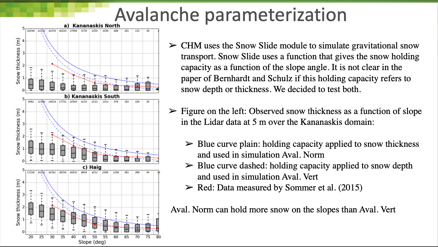
SnowSlide is a simple topographically-driven model that simulates the effects of gravitational snow transport. It uses a snow holding depth that decreases exponentially with increasing slope angle, limiting snow accumulation in steep terrain. The algorithm moves mass from the highest triangle of the mesh to the lowest one. If the snow depth exceeds the snow holding capacity for a given triangle, excess snow is redistributed to the lower adjacent triangles, proportionally to the elevation difference between the neighboring triangles and the original one. SnowSlide uses the total elevation (snow depth plus surface elevation) to operate. In this study, the default formulation of the snow holding depth proposed by Bernhardt and Schulz (2010) is used which leads to a maximal snow thickness (taken perpendicular to the slope) of 3.08 m, 1.11 m, 0.45 m, and 0.15 m for slopes of 30° 45°, 60°, and 75°, respectively.

In the manuscript it is unclear if the holding capacity (max depth) is parameterized for a snow thickness normal to the slope (i.e., how the snowmodels treat snow) or if it is in the vertical direction (i.e., how LiDAR would measure it, a.k.a cosine corrected snow depth). An analysis versus observed LiDAR derived snowdepths over the Kananaskis, Canada domain as well as data observed by Sommer et al. (2015) showed a better evaluation with snowdepths if it is assumed the parameterization is defined for snowdepths in the vertical.

Depends:

• Snow depth “snowdepthavg” [m]

• Snow depth “snowdepthavg_vert” [m]

• Snow Water Equivalent “swe” [mm]

Provides:

• Change in snow mass due to avalanching “delta_avalanche_mass” [mm]

• Change in snow depth due to avalanching “delta_avalanche_snowdepth” [mm]

• Maximum snowdepth holding capacity of a triangle “maxDepth” [m]

Configuration:

 {
    "avalache_mult": 3178.4,
    "avalache_pow": -1.998
}

avalache_mult

avalache_pow

References:

• Bernhardt, M., Schulz, K. (2010). SnowSlide: A simple routine for calculating gravitational snow transport Geophysical Research Letters 37(11), 1-6. https://dx.doi.org/10.1029/2010gl043086

Default:

3178.4

Default:

-1.998

Lehning_snowpack

class Lehning_snowpack : public module_base

SNOWPACK (Bartelt and Lehning, 2002) is a multilayer finite-element energy balance snow model originally developed for avalanche hazard forecasting. It has the greatest computational burden of all snowpack models in CHM. This version of SNOWPACK has been modified to allow unlimited removal of snow layers by the blowing snow and avalanche routines.

Depends:

• Incoming shortwave radiation, all beams “iswr” [ \( W \cdot m^{-2} \) ]

• Incomging longwave radiation “ilwr” [ \( W \cdot m^{-2} \) ]

• Relative humidity “rh” [%]

• Air temperature “t” [ \( {}^\circ C \)]

• Windspeed at 2m “U_2m_above_srf” [ \( m \cdot s^{-1} \)]

• Precipitation “p” [ \( mm \cdot dt^{-1} \)]

• Precipitation rain fraction “frac_precip_rain” [-]

• Snow albedo “snow_albedo” [-]

Optional:

• Optionally, depend on the _subcanopy variants of the above

• Blowing snow erosion/deposition mass “drift_mass” [mm]

• Ground temperature “T_g” [ \( {}^\circ C \)]

Provides:

• Change in internal energy “dQ” [ \( W \cdot m^{-2} \) ]

• Snow water equivalent “swe” [mm]

• Bulk snow temperature “T_s” [ \( {}^\circ C \)]

• Surface exchange layer temperature “T_s_0”

• Number of discretization nodes “n_nodes”

• Number of discretization layers “n_elem”

• Snowdepth “snowdepthavg” [m]

• Sensible heat flux “H” [ \( W \cdot m^{-2} \) ]

• Latent heat flux “E” [ \( W \cdot m^{-2} \) ]

• Ground heat flux “G” [ \( W \cdot m^{-2} \) ]

• Outgoing longwave radiation “ilwr_out” [ \( W \cdot m^{-2} \) ]

• Reflected shortwave radiation “iswr_out” [ \( W \cdot m^{-2} \) ]

• Net allwave radiation “R_n” [ \( W \cdot m^{-2} \) ]

• Snowpack runoff “runoff” [mm]

• Snow mass removed “mass_snowpack_removed” [mm]

• Total snowpack runoff “sum_runoff”

• Total surface sublimation loss “sum_subl”

• Sublimation loss “sublimation”

• Evaporation loss “evap”

• ”MS_SWE”

• ”MS_WATER”

• ”MS_TOTALMASS”

• ”MS_SOIL_RUNOFF”

Configuration:

{
   "sno":
   {
      "SoilAlbedo": 0.09,
      "BareSoil_z0": 0.2,
      "WindScalingFactor": 1,
      "TimeCountDeltaHS": 0.0  
   }

Note

Currently SNOWPACK is setup to be run an external albedo model and should be changed to default back to the SNOWPACK one.

threshold_p_phase

class threshold_p_phase : public module_base

Calculates phase from air temperature. Defaults to 2 \( {}^\circ C \), looks for the config parameter “threshold_temperature”. Binary snow/rain at 2 \( {}^\circ C \) threshold.

Depends:

• Air temperature “t” [ \( {}^\circ C \) ]

• Precipitation “p” [ \( mm \cdot dt^{-1} \) ]

Provides:

• Fractional precipitation that is rain “frac_precip_rain” [0-1]

• Fractional precipitation that is snow “frac_precip_snow” [0-1]

• Precipitation, rain “p_rain” [ \( mm \cdot dt^{-1} \)]

• Precipitation, snow “p_snow” [ \( mm \cdot dt^{-1} \)]

Configuration:

{
   "threshold_temperature": 2.0
}

threshold_temperature

Threshold air temperature for rain/snow delineation

Default:

2.0 \({}^\circ C\)

Soil Infiltration

Gray_inf

class Gray_inf : public module_base

Estimates areal snowmelt infiltration into frozen soils for: a) Restricted - Water entry impeded by surface conditions b) Limited - Capiliary flow dominates and water flow influenced by soil physical properties c) Unlimited - Gravity flow dominates

Depends:

• Snow water equivalent “swe” [mm]

• Snow melt for interval “snowmelt_int” [ \(mm \cdot dt^{-1}\)]

Provides:

• Infiltration “inf” [ \(mm \cdot dt^{-1}\)]

• Total infiltration “total_inf” [mm]

• Total infiltration excess “total_excess” [mm]

• Total runoff “runoff” [mm]

• Total soil storage “soil_storage”

• Potential infiltration “potential_inf”

• Opportunity time for infiltration to occur “opportunity_time”

• Available storage for water of the soil “available_storage”

References:

• Gray, D., Toth, B., Zhao, L., Pomeroy, J., Granger, R. (2001). Estimating areal snowmelt infiltration into frozen soils Hydrological Processes 15(16), 3095-3111. https://dx.doi.org/10.1002/hyp.320

Note

Has hardcoded soil parameters that need to be read from the mesh parameters.

Uncategorized

module_template

class module_template : public module_base

Template header file for new module implementations.

Depends:

Provides:

mpi

class mpi : public module_base

MPI usage example

Depends:

• None

Provides:

• None

Configuration:

• None

Parameters:

• None

Wind

fetchr

class fetchr : public module_base

Calculates upwind fetch distances. The fetch is broken if a triangle at distance d * I > current triangle’s elevation.

Depends:

• Wind direction “vw_dir” [degrees]

Provides:

• Fetch distance “fetch” [m]

Configuration:

{
   "steps": 10,
   "max_distance": 1000
}

steps

Number of steps along the search vector to check for a higher point

max_distance

Maximum search distance to look for a higher point

I

Rise/run threshold to multiply against the distance of a test triangle.

References:

• Lapen, D. R., and L. W. Martz (1993), The measurement of two simple topographic indices of wind sheltering-exposure from raster digital elevation models, Comput. Geosci., 19(6), 769–779, doi:10.1016/0098-3004(93)90049-B.

Type:

int

Default:

10

Type:

double

Default:

1000 m

Type:

double

Default:

0.06

Liston_wind

class Liston_wind : public module_base

Calculates windspeeds using a terrain curvature following Liston and Elder 2006. Direction convention is (North = 0, clockwise from North)

Depends from met:

• Wind at reference height “U_R” [ \(m \cdot s^{-1}\)]

• Direction at reference height ‘vw_dir’ [degrees] (North = 0, clockwise from North)

Provides:

• Wind at reference height “U_R”

• Interpolated wind field at reference height prior to downscaling “U_R_orig” [ \(m \cdot s^{-1}\)]

• Wind direction “vw_dir” [degrees]

• Original wind direction “vw_dir_orig” [degrees]

• Amount the wind vector direction has been changed “vw_dir_divergence” [degrees]

• Zonal U at reference height “zonal_u” [ \( m \cdot s^{-1}\) ]

• Zonal V at reference height “zonal_v” [ \( m \cdot s^{-1}\) ]

Configuration:

{
   "distance": 300,
   "Ww_coeff: 1,
   "ys": 0.5,
   "yc": 0.5
}

distance

Distance to “look” to compute the terrain curvature.

Ww_coeff

Leading coefficient in equation 16. Used for compatibility with calibration approach such as done by Pohl.

ys

Slope weight. Valid range [0,1]. The value of 0.5 gives equal weight to slope and curvature

yc

Curvature weight. Valid range [0,1]. The value of 0.5 gives equal weight to slope and curvature

References:

Liston, G. E., & Elder, K. (2006). A meteorological distribution system for high-resolution terrestrial modeling (MicroMet). Journal of Hydrometeorology, 7(2), 217–234. http://doi.org/10.1175/JHM486.1

Type:

double

Default:

300

Type:

int

Default:

1

Type:

double

Default:

0.5

Type:

double

Default:

0.5

MS_wind

class MS_wind : public module_base

Calculates windspeeds using the Mason Sykes wind speed from Essery, et al (1999), using 8 lookup map from DBSM. Optionally uses Ryan, et al. for wind direction correction.

Depends from met:

• Wind at reference height “U_R” [ \( m \cdot s^{-1}\) ]

• Direction at reference height “vw_dir” [degrees]

Provides:

• Wind speed at reference height “U_R” [ \( m \cdot s^{-1}\) ]

• Wind direction ‘vw_dir’ at reference height [degrees]

• Speedup magnitude “W_speedup” [-]

• Zonal u speed component at 2m “2m_zonal_u” [ \( m \cdot s^{-1}\) ]

• Zonal v speed component at 2m “2m_zonal_v” [ \( m \cdot s^{-1}\) ]

• Original interpolated wind direction “vw_dir_orig” [degrees]

Parameters:

Requires speedup, u, and v parameters named “MS%i_U” and “MS%i_V” and “MS%i” for each of the 8 directions. These need to be generated using DBSM in tools/MSwind.

Configuration:

{
   "speedup_height": 2.0,
   "use_ryan_dir", false
}

speedup_height

The height at which the MS Wind tool was run for. The default is 2 m and shouldn’t be changed.

use_ryan_dir

Instead of using the _u and _v components to compute direction perturbation, use the algorithm of Ryan as per Liston and Elder (2006)

Reference:

Essery, R., Li, L., Pomeroy, J. (1999). A distributed model of blowing snow over complex terrain Hydrological Processes 13(), 2423-2438.

Type:

double

Default:

2.0

Type:

boolean

Default:

false

uniform_wind

class uniform_wind : public module_base

Spatially interpolates wind speed and direction without any terrain speed-up modification

Depends from met:

• Wind at reference height “U_R” [ \( m \cdot s^{-1}\) ]

• Direction at reference height “vw_dir” [degrees]

Provides:

• Wind speed at reference height “U_R” [ \( m \cdot s^{-1}\) ]

• Wind direction ‘vw_dir’ at reference height [degrees]

WindNinja

class WindNinja : public module_base

Calculates wind speed and direction following the downscaling stategy of Barcons et al. (2018). This is via a library of high-resolution wind field generated with the WindNinja wind flow model. Unless the reference height windspeed is provided, use the scale_wind_speed filter to log-scale the windspeed up to U_R.

Depends from met:

• Wind at reference height “U_R” [ \( m \cdot s^{-1}\) ]

• Direction at reference height “vw_dir” [degrees]

Provides:

• Wind speed at reference height “U_R” [ \( m \cdot s^{-1}\) ]

• Wind direction ‘vw_dir’ at reference height [degrees]

• Zonal U at reference height “zonal_u” [ \( m \cdot s^{-1}\) ]

• Zonal V at reference height “zonal_v” [ \( m \cdot s^{-1}\) ]

Diagnostics:

• Downscaled windspeed “Ninja_speed” [ \( m \cdot s^{-1}\) ]

• Interpolated wind field at reference height prior to downscaling “U_R_orig” [ \(m \cdot s^{-1}\)]

• Interpolated zonal U at level H_Forc “interp_zonal_u” [ \( m \cdot s^{-1}\) ]

• Interpolated zonal V at level H_Forc “interp_zonal_v” [ \( m \cdot s^{-1}\) ]

• What lookup map was used “lookup_d” [-]

• Original wind direction “vw_dir_orig” [degrees]

• Amount the wind vector direction has been changed “vw_dir_divergence” [degrees]

Configuration:

{
   "ninja_average": true,
   "compute_Sx": true,
   "ninja_recirc": false,
   "Sx_crit", 30.
   "L_avg": 1000.
   "H_forc": 40,
   "Max_spdup": 3.0,
   "Min_spdup": 0.1,
}

ninja_average

Linear interpolation between the closest 2 wind fields from the library

compute_Sx

Use the Winstral Sx parameterization to idenitify and modify lee-side windfield. This will cause a runtime error (conflict) if Winstral_parameters is also a module. This uses an angular window of 30 degrees and a step size of 10 m.

ninja_recirc

Enables the leeside slow down via compute_Sx. Requires "compute_Sx":true.

Sx_crit

Reduce wind speed on the lee side of mountain crest identified by Sx>Sx_crit

..confval:: L_avg

The WindMapper tool uses a radius to compute a mean. This is the length over which that average is done. Normally this will be baked into the parameter name (e.g., Ninja_1000). However, there may be reasons to specifiy it directly. Cannot be used if the parameters have the _Lavg suffix. You likely don’t need to set this.

H_forc

Max_spdup

Limit speed up value to Max_spdup to avoid unrelistic values at crest top

Min_spdup

Limit speed up value to Max_spdup to avoid unrelistic values at crest top

Parameters:

Requires speedup, u, and v parameters named “Ninja%i_U” and “Ninja%i_V” and “Ninja%i” for each of the n directions. Should be generated with WindMapper. The number of directions will be automatically determined as will the Lavg value. These should be computed with the Windmapper tool .

References:

• Barcons, J., Avila, M., Folch, A. (2018). A wind field downscaling strategy based on domain segmentation and transfer functions Wind Energy 21(6)https://dx.doi.org/10.1002/we.2169

Type:

boolean

Default:

true

Type:

boolean

Default:

true

Type:

boolean

Default:

false

Type:

double

Default:

Type:

int

Default:

None

Type:

double

Default:

40.0

Reference height for input forcing and WindNinja wind field library

Type:

double

Default:

3.0

Type:

double

Default:

3.0

scale_wind_vert

class scale_wind_vert : public module_base

Scales wind speed from reference height to defined heights. Scales the wind vertically using a neutral stability log relationship. If snow depth is present, the height is taken into account. A fixed z0 of 0.01m is currently used. If a canopy is present then an exp sub-canopy scaling is used.

Depends:

• Wind speed @reference height “U_R” [ \( m \cdot s^{-1} \) ]

Optional:

• Snow depth to take into account for the scaling “snowdepthavg” [m]

Provides:

• Wind speed @2m “U_2m_above_srf” [ \( m \cdot s^{-1} \) ]

Parameters:

• If ignore_canopy=False, then Leaf Area Index “LAI” [-]

Configuration:

{
   "ignore_canopy": false
}

ignore_canopy

Ignores the vegetation canopy

Default:

false

By provides variable

Note

These provides are automatically produced from the module code. They do not include provides that are dynamically generated

i.e., provides("t_"+some_var);

2m_zonal_u

MS_wind

class MS_wind : public module_base

Calculates windspeeds using the Mason Sykes wind speed from Essery, et al (1999), using 8 lookup map from DBSM. Optionally uses Ryan, et al. for wind direction correction.

Depends from met:

• Wind at reference height “U_R” [ \( m \cdot s^{-1}\) ]

• Direction at reference height “vw_dir” [degrees]

Provides:

• Wind speed at reference height “U_R” [ \( m \cdot s^{-1}\) ]

• Wind direction ‘vw_dir’ at reference height [degrees]

• Speedup magnitude “W_speedup” [-]

• Zonal u speed component at 2m “2m_zonal_u” [ \( m \cdot s^{-1}\) ]

• Zonal v speed component at 2m “2m_zonal_v” [ \( m \cdot s^{-1}\) ]

• Original interpolated wind direction “vw_dir_orig” [degrees]

Parameters:

Requires speedup, u, and v parameters named “MS%i_U” and “MS%i_V” and “MS%i” for each of the 8 directions. These need to be generated using DBSM in tools/MSwind.

Configuration:

{
   "speedup_height": 2.0,
   "use_ryan_dir", false
}

speedup_height

The height at which the MS Wind tool was run for. The default is 2 m and shouldn’t be changed.

use_ryan_dir

Instead of using the _u and _v components to compute direction perturbation, use the algorithm of Ryan as per Liston and Elder (2006)

Reference:

Essery, R., Li, L., Pomeroy, J. (1999). A distributed model of blowing snow over complex terrain Hydrological Processes 13(), 2423-2438.

Type:

double

Default:

2.0

Type:

boolean

Default:

false

2m_zonal_v

MS_wind

class MS_wind : public module_base

Calculates windspeeds using the Mason Sykes wind speed from Essery, et al (1999), using 8 lookup map from DBSM. Optionally uses Ryan, et al. for wind direction correction.

Depends from met:

• Wind at reference height “U_R” [ \( m \cdot s^{-1}\) ]

• Direction at reference height “vw_dir” [degrees]

Provides:

• Wind speed at reference height “U_R” [ \( m \cdot s^{-1}\) ]

• Wind direction ‘vw_dir’ at reference height [degrees]

• Speedup magnitude “W_speedup” [-]

• Zonal u speed component at 2m “2m_zonal_u” [ \( m \cdot s^{-1}\) ]

• Zonal v speed component at 2m “2m_zonal_v” [ \( m \cdot s^{-1}\) ]

• Original interpolated wind direction “vw_dir_orig” [degrees]

Parameters:

Requires speedup, u, and v parameters named “MS%i_U” and “MS%i_V” and “MS%i” for each of the 8 directions. These need to be generated using DBSM in tools/MSwind.

Configuration:

{
   "speedup_height": 2.0,
   "use_ryan_dir", false
}

speedup_height

The height at which the MS Wind tool was run for. The default is 2 m and shouldn’t be changed.

use_ryan_dir

Instead of using the _u and _v components to compute direction perturbation, use the algorithm of Ryan as per Liston and Elder (2006)

Reference:

Essery, R., Li, L., Pomeroy, J. (1999). A distributed model of blowing snow over complex terrain Hydrological Processes 13(), 2423-2438.

Type:

double

Default:

2.0

Type:

boolean

Default:

false

E

FSM

class FSM : public module_base

Flexible Snow Model (FSM) 2.0

“The Flexible Snow Model (FSM2) is a multi-physics energy balance model of snow accumulation and melt,

extending the Factorial Snow Model (Essery, 2015) with additional physics, driving and output options.”

This version of FSM has been customized to have the sophisticated process parametrizations selected in every case, except atmospheric stability corrections.

Depends:

• Solar elevation “solar_el” [degrees]

• Incoming longwave radiation “ilwr” \([W \cdot m^{-2}\)]

• Relative Humidy “rh” [%]

• Air temperature “t” [ \( {}^\circ C \)]

• Precipitation snow “p_snow” [ \(mm \cdot dt^{-1}\)]

• Precipitation rain “p_rain” [ \(mm \cdot dt^{-1}\)]

• Wind speed 2 m above surface “U_2m_above_srf” [ \( m \cdot s^{-1}\) ]

• Incoming shortwave radiation, direct beam “iswr_direct” \([W \cdot m^{-2}\)]

• Incoming shortwave radiation, diffuse beam “iswr_diffuse” \([W \cdot m^{-2}\)]

Provides:

• Snow Water Equivalent “swe” [mm]

• Snow depth “snowdepthavg” [m]

• Snow depth slope corrected “snowdepthavg_vert” [m]

Optional:

Sub-canopy forcing:

• Subcanopy incoming shortwave radiation “iswr_subcanopy” \([W \cdot m^{-2}\)]

• Subcanopy relative humidity “rh_subcanopy” [%]

• Subcanopy air temperatue “ta_subcanopy” [ \( {}^\circ C \)]

• Subcanopy incoming longwave radidation “ilwr_subcanopy” \([W \cdot m^{-2}\)]

References:

• https://github.com/RichardEssery/FSM2

• Essery, R. (2015). A factorial snowpack model (FSM 1.0) Geoscientific Model Development 8(12), 3867 3876. https://dx.doi.org/10.5194/gmd-8-3867-2015

Warning

Snow transport and vegetation characteristics remain a TODO

snobal

class snobal : public module_base

Snobal is a physically-based snowpack model that approximates the snowpack with two layers. The surface-active layer has a fixed thickness of 0.1 m and is used to estimate surface temperature for outgoing longwave radiation and turbulent heat fluxes. The second lower layer represents the remaining snowpack. For each layer, Snobal simulates the evolution of the snow water equivalent, temperature, density, cold content, and liquid water content. This version of Snobal includes an improved algorithm for snow compaction that accounts for bulk compaction and temperature metamorphism (Hedrick et al., 2018).

Depends:

• Incoming shortwave radiation, all beams “iswr” [ \( W \cdot m^{-2} \) ]

• Incomging longwave radiation “ilwr” [ \( W \cdot m^{-2} \) ]

• Relative humidity “rh” [%]

• Air temperature “t” [ \( {}^\circ C \)]

• Windspeed at 2m “U_2m_above_srf” [ \( m \cdot s^{-1} \)]

• Precipitation “p” [ \( mm \cdot dt^{-1} \)]

• Precipitation snow fraction “frac_precip_snow” [-]

• Snow albedo “snow_albedo” [-]

Optional:

• Optionally, depend on the _subcanopy variants of the above

• Blowing snow erosion/deposition mass “drift_mass” [mm]

• Ground temperature “T_g” [ \( {}^\circ C \)]

• Change in snow mass due to avalanching “delta_avalanche_mass” [mm]

• Change in snow depth due to avalanching “delta_avalanche_snowdepth” [mm]

Provides:

• Snow water equivalent “swe” [mm]

• Interval snowmelt “snowmelt_int” [mm]

• Net allwave radiation “R_n” [ \( W \cdot m^{-2} \) ]

• Sensible heat flux “H” [ \( W \cdot m^{-2} \) ]

• Latent heat flux “E” [ \( W \cdot m^{-2} \) ]

• Ground heat flux “G” [ \( W \cdot m^{-2} \) ]

• Advected heat from precipitation “M” [ \( W \cdot m^{-2} \) ]

• Change in internal energy “dQ” [ \( W \cdot m^{-2} \) ]

• Cold content of entire snowpack “cc” [ \( J \cdot m^{-2} \) ]

• Bulk snow temperature “T_s” [K]

• Surface exchange layer temperature “T_s_0” [K]

• Lower layer temperature “T_s_l” [K]

• Was an iteration error hit “dead”. Diagnostic, don’t use. [-]

• Net shortwave radiation at the surface. Diagnostic. “iswr_out” [ \( W \cdot m^{-2} \) ]

• Binary is the snow isothermal “isothermal” [0,1]

• Outgoing longwave radiation “ilwr_out” [ \( W \cdot m^{-2} \) ]

• Total snowpack runoff “sum_snowpack_runoff”

• Total snowpack sublimation “sum_snowpack_subl”

• Total precipitation onto the snowpack. Diagnostic. “sum_snowpack_pcp” [mm]

• Total snowpack melt “sum_melt” [mm]

• Snowdepth “snowdepthavg” [m]

• Snowdepth in the vertical direction (cosine corrected) “snowdepthavg_vert” [m]

Configuration:

{
   "drift_density": 300,
   "const_T_g": -4.0,
   "use_slope_SWE": true,
   "param_snow_compaction": 1,
   "max_h2o_vol":0.0001,
   "kt_wetsand": 0.08,
   "max_active_layer": 0.1,
   "z0":0.001,
   "z_T":2.6,
   "z_u":2.96,
   "z_g":0.1,
}

drift_density

Density of snow that is added from drift events

const_T_g

Constant ground temperature

use_slope_SWE

Use slope corrected snowdepth for compaction. I.e., parallel to gravity force.

param_snow_compaction

Set to 1 to use new Hedrick, et al parameterization for snow compaction. 0 for origianl Snobal.

max_h2o_vol

Maximum volumetric water content in the snow. Tends to be required to be set quite low.

kt_wetsand

Thermal conductivity of wet sand for G flux

max_active_layer

Thickness of active layer

z0

Rouighness length

z_T

Height of air temperature

z_u

Height of wind measurement

z_g

Depth of ground temperature measurement

References:

• Marks, D., Domingo, J., Susong, D., Link, T., Garen, D. (1999). A spatially distributed energy balance snowmelt model for application in mountain basins Hydrological Processes 13(12-13), 1935-1959.

• Hedrick, A., Marks, D., Havens, S., Robertson, M., Johnson, M., Sandusky, M., Marshall, H., Kormos, P., Bormann, K., Painter, T. (2018). Direct Insertion of NASA Airborne Snow Observatory‐Derived Snow Depth Time Series Into the iSnobal Energy Balance Snow Model Water Resources Research 54(10), 8045-8063. https://dx.doi.org/10.1029/2018wr023190

Default:

300 \(kg \cdot m^3\)

Default:

-4.0 \({}^\circ C\)

Default:

true

Default:

1

Default:

0.0001

Default:

\(0.08 W \cdot m^{-2}\)

Default:

0.1 m

Default:

0.001 m

Default:

2.6 m

Default:

2 m

Default:

0.1

Lehning_snowpack

class Lehning_snowpack : public module_base

SNOWPACK (Bartelt and Lehning, 2002) is a multilayer finite-element energy balance snow model originally developed for avalanche hazard forecasting. It has the greatest computational burden of all snowpack models in CHM. This version of SNOWPACK has been modified to allow unlimited removal of snow layers by the blowing snow and avalanche routines.

Depends:

• Incoming shortwave radiation, all beams “iswr” [ \( W \cdot m^{-2} \) ]

• Incomging longwave radiation “ilwr” [ \( W \cdot m^{-2} \) ]

• Relative humidity “rh” [%]

• Air temperature “t” [ \( {}^\circ C \)]

• Windspeed at 2m “U_2m_above_srf” [ \( m \cdot s^{-1} \)]

• Precipitation “p” [ \( mm \cdot dt^{-1} \)]

• Precipitation rain fraction “frac_precip_rain” [-]

• Snow albedo “snow_albedo” [-]

Optional:

• Optionally, depend on the _subcanopy variants of the above

• Blowing snow erosion/deposition mass “drift_mass” [mm]

• Ground temperature “T_g” [ \( {}^\circ C \)]

Provides:

• Change in internal energy “dQ” [ \( W \cdot m^{-2} \) ]

• Snow water equivalent “swe” [mm]

• Bulk snow temperature “T_s” [ \( {}^\circ C \)]

• Surface exchange layer temperature “T_s_0”

• Number of discretization nodes “n_nodes”

• Number of discretization layers “n_elem”

• Snowdepth “snowdepthavg” [m]

• Sensible heat flux “H” [ \( W \cdot m^{-2} \) ]

• Latent heat flux “E” [ \( W \cdot m^{-2} \) ]

• Ground heat flux “G” [ \( W \cdot m^{-2} \) ]

• Outgoing longwave radiation “ilwr_out” [ \( W \cdot m^{-2} \) ]

• Reflected shortwave radiation “iswr_out” [ \( W \cdot m^{-2} \) ]

• Net allwave radiation “R_n” [ \( W \cdot m^{-2} \) ]

• Snowpack runoff “runoff” [mm]

• Snow mass removed “mass_snowpack_removed” [mm]

• Total snowpack runoff “sum_runoff”

• Total surface sublimation loss “sum_subl”

• Sublimation loss “sublimation”

• Evaporation loss “evap”

• ”MS_SWE”

• ”MS_WATER”

• ”MS_TOTALMASS”

• ”MS_SOIL_RUNOFF”

Configuration:

{
   "sno":
   {
      "SoilAlbedo": 0.09,
      "BareSoil_z0": 0.2,
      "WindScalingFactor": 1,
      "TimeCountDeltaHS": 0.0  
   }

Note

Currently SNOWPACK is setup to be run an external albedo model and should be changed to default back to the SNOWPACK one.

ET

PenmanMonteith_evaporation

class PenmanMonteith_evaporation : public module_base

Calculates evapo-transpiration via Penman-Monteith.

Not currently maintained.

Depends:

• Incoming shortwave radaition “iswr” [ \( W \cdot m^{-2} \) ]

• Incoming longwave radiation “ilwr” [ \( W \cdot m^{-2} \) ]

• Relative humidity “rh” [%]

• Windspeed at 2m “U_2m_above_srf” [ \( m \cdot s^{-1} \) ]

Provides:

• Evapotranspiration “ET” [ \( mm \cdot dt^{-1} \) ]

G

snobal

class snobal : public module_base

Snobal is a physically-based snowpack model that approximates the snowpack with two layers. The surface-active layer has a fixed thickness of 0.1 m and is used to estimate surface temperature for outgoing longwave radiation and turbulent heat fluxes. The second lower layer represents the remaining snowpack. For each layer, Snobal simulates the evolution of the snow water equivalent, temperature, density, cold content, and liquid water content. This version of Snobal includes an improved algorithm for snow compaction that accounts for bulk compaction and temperature metamorphism (Hedrick et al., 2018).

Depends:

• Incoming shortwave radiation, all beams “iswr” [ \( W \cdot m^{-2} \) ]

• Incomging longwave radiation “ilwr” [ \( W \cdot m^{-2} \) ]

• Relative humidity “rh” [%]

• Air temperature “t” [ \( {}^\circ C \)]

• Windspeed at 2m “U_2m_above_srf” [ \( m \cdot s^{-1} \)]

• Precipitation “p” [ \( mm \cdot dt^{-1} \)]

• Precipitation snow fraction “frac_precip_snow” [-]

• Snow albedo “snow_albedo” [-]

Optional:

• Optionally, depend on the _subcanopy variants of the above

• Blowing snow erosion/deposition mass “drift_mass” [mm]

• Ground temperature “T_g” [ \( {}^\circ C \)]

• Change in snow mass due to avalanching “delta_avalanche_mass” [mm]

• Change in snow depth due to avalanching “delta_avalanche_snowdepth” [mm]

Provides:

• Snow water equivalent “swe” [mm]

• Interval snowmelt “snowmelt_int” [mm]

• Net allwave radiation “R_n” [ \( W \cdot m^{-2} \) ]

• Sensible heat flux “H” [ \( W \cdot m^{-2} \) ]

• Latent heat flux “E” [ \( W \cdot m^{-2} \) ]

• Ground heat flux “G” [ \( W \cdot m^{-2} \) ]

• Advected heat from precipitation “M” [ \( W \cdot m^{-2} \) ]

• Change in internal energy “dQ” [ \( W \cdot m^{-2} \) ]

• Cold content of entire snowpack “cc” [ \( J \cdot m^{-2} \) ]

• Bulk snow temperature “T_s” [K]

• Surface exchange layer temperature “T_s_0” [K]

• Lower layer temperature “T_s_l” [K]

• Was an iteration error hit “dead”. Diagnostic, don’t use. [-]

• Net shortwave radiation at the surface. Diagnostic. “iswr_out” [ \( W \cdot m^{-2} \) ]

• Binary is the snow isothermal “isothermal” [0,1]

• Outgoing longwave radiation “ilwr_out” [ \( W \cdot m^{-2} \) ]

• Total snowpack runoff “sum_snowpack_runoff”

• Total snowpack sublimation “sum_snowpack_subl”

• Total precipitation onto the snowpack. Diagnostic. “sum_snowpack_pcp” [mm]

• Total snowpack melt “sum_melt” [mm]

• Snowdepth “snowdepthavg” [m]

• Snowdepth in the vertical direction (cosine corrected) “snowdepthavg_vert” [m]

Configuration:

{
   "drift_density": 300,
   "const_T_g": -4.0,
   "use_slope_SWE": true,
   "param_snow_compaction": 1,
   "max_h2o_vol":0.0001,
   "kt_wetsand": 0.08,
   "max_active_layer": 0.1,
   "z0":0.001,
   "z_T":2.6,
   "z_u":2.96,
   "z_g":0.1,
}

drift_density

Density of snow that is added from drift events

const_T_g

Constant ground temperature

use_slope_SWE

Use slope corrected snowdepth for compaction. I.e., parallel to gravity force.

param_snow_compaction

Set to 1 to use new Hedrick, et al parameterization for snow compaction. 0 for origianl Snobal.

max_h2o_vol

Maximum volumetric water content in the snow. Tends to be required to be set quite low.

kt_wetsand

Thermal conductivity of wet sand for G flux

max_active_layer

Thickness of active layer

z0

Rouighness length

z_T

Height of air temperature

z_u

Height of wind measurement

z_g

Depth of ground temperature measurement

References:

• Marks, D., Domingo, J., Susong, D., Link, T., Garen, D. (1999). A spatially distributed energy balance snowmelt model for application in mountain basins Hydrological Processes 13(12-13), 1935-1959.

• Hedrick, A., Marks, D., Havens, S., Robertson, M., Johnson, M., Sandusky, M., Marshall, H., Kormos, P., Bormann, K., Painter, T. (2018). Direct Insertion of NASA Airborne Snow Observatory‐Derived Snow Depth Time Series Into the iSnobal Energy Balance Snow Model Water Resources Research 54(10), 8045-8063. https://dx.doi.org/10.1029/2018wr023190

Default:

300 \(kg \cdot m^3\)

Default:

-4.0 \({}^\circ C\)

Default:

true

Default:

1

Default:

0.0001

Default:

\(0.08 W \cdot m^{-2}\)

Default:

0.1 m

Default:

0.001 m

Default:

2.6 m

Default:

2 m

Default:

0.1

Lehning_snowpack

class Lehning_snowpack : public module_base

SNOWPACK (Bartelt and Lehning, 2002) is a multilayer finite-element energy balance snow model originally developed for avalanche hazard forecasting. It has the greatest computational burden of all snowpack models in CHM. This version of SNOWPACK has been modified to allow unlimited removal of snow layers by the blowing snow and avalanche routines.

Depends:

• Incoming shortwave radiation, all beams “iswr” [ \( W \cdot m^{-2} \) ]

• Incomging longwave radiation “ilwr” [ \( W \cdot m^{-2} \) ]

• Relative humidity “rh” [%]

• Air temperature “t” [ \( {}^\circ C \)]

• Windspeed at 2m “U_2m_above_srf” [ \( m \cdot s^{-1} \)]

• Precipitation “p” [ \( mm \cdot dt^{-1} \)]

• Precipitation rain fraction “frac_precip_rain” [-]

• Snow albedo “snow_albedo” [-]

Optional:

• Optionally, depend on the _subcanopy variants of the above

• Blowing snow erosion/deposition mass “drift_mass” [mm]

• Ground temperature “T_g” [ \( {}^\circ C \)]

Provides:

• Change in internal energy “dQ” [ \( W \cdot m^{-2} \) ]

• Snow water equivalent “swe” [mm]

• Bulk snow temperature “T_s” [ \( {}^\circ C \)]

• Surface exchange layer temperature “T_s_0”

• Number of discretization nodes “n_nodes”

• Number of discretization layers “n_elem”

• Snowdepth “snowdepthavg” [m]

• Sensible heat flux “H” [ \( W \cdot m^{-2} \) ]

• Latent heat flux “E” [ \( W \cdot m^{-2} \) ]

• Ground heat flux “G” [ \( W \cdot m^{-2} \) ]

• Outgoing longwave radiation “ilwr_out” [ \( W \cdot m^{-2} \) ]

• Reflected shortwave radiation “iswr_out” [ \( W \cdot m^{-2} \) ]

• Net allwave radiation “R_n” [ \( W \cdot m^{-2} \) ]

• Snowpack runoff “runoff” [mm]

• Snow mass removed “mass_snowpack_removed” [mm]

• Total snowpack runoff “sum_runoff”

• Total surface sublimation loss “sum_subl”

• Sublimation loss “sublimation”

• Evaporation loss “evap”

• ”MS_SWE”

• ”MS_WATER”

• ”MS_TOTALMASS”

• ”MS_SOIL_RUNOFF”

Configuration:

{
   "sno":
   {
      "SoilAlbedo": 0.09,
      "BareSoil_z0": 0.2,
      "WindScalingFactor": 1,
      "TimeCountDeltaHS": 0.0  
   }

Note

Currently SNOWPACK is setup to be run an external albedo model and should be changed to default back to the SNOWPACK one.

H

FSM

class FSM : public module_base

Flexible Snow Model (FSM) 2.0

“The Flexible Snow Model (FSM2) is a multi-physics energy balance model of snow accumulation and melt,

extending the Factorial Snow Model (Essery, 2015) with additional physics, driving and output options.”

This version of FSM has been customized to have the sophisticated process parametrizations selected in every case, except atmospheric stability corrections.

Depends:

• Solar elevation “solar_el” [degrees]

• Incoming longwave radiation “ilwr” \([W \cdot m^{-2}\)]

• Relative Humidy “rh” [%]

• Air temperature “t” [ \( {}^\circ C \)]

• Precipitation snow “p_snow” [ \(mm \cdot dt^{-1}\)]

• Precipitation rain “p_rain” [ \(mm \cdot dt^{-1}\)]

• Wind speed 2 m above surface “U_2m_above_srf” [ \( m \cdot s^{-1}\) ]

• Incoming shortwave radiation, direct beam “iswr_direct” \([W \cdot m^{-2}\)]

• Incoming shortwave radiation, diffuse beam “iswr_diffuse” \([W \cdot m^{-2}\)]

Provides:

• Snow Water Equivalent “swe” [mm]

• Snow depth “snowdepthavg” [m]

• Snow depth slope corrected “snowdepthavg_vert” [m]

Optional:

Sub-canopy forcing:

• Subcanopy incoming shortwave radiation “iswr_subcanopy” \([W \cdot m^{-2}\)]

• Subcanopy relative humidity “rh_subcanopy” [%]

• Subcanopy air temperatue “ta_subcanopy” [ \( {}^\circ C \)]

• Subcanopy incoming longwave radidation “ilwr_subcanopy” \([W \cdot m^{-2}\)]

References:

• https://github.com/RichardEssery/FSM2

• Essery, R. (2015). A factorial snowpack model (FSM 1.0) Geoscientific Model Development 8(12), 3867 3876. https://dx.doi.org/10.5194/gmd-8-3867-2015

Warning

Snow transport and vegetation characteristics remain a TODO

snobal

class snobal : public module_base

Snobal is a physically-based snowpack model that approximates the snowpack with two layers. The surface-active layer has a fixed thickness of 0.1 m and is used to estimate surface temperature for outgoing longwave radiation and turbulent heat fluxes. The second lower layer represents the remaining snowpack. For each layer, Snobal simulates the evolution of the snow water equivalent, temperature, density, cold content, and liquid water content. This version of Snobal includes an improved algorithm for snow compaction that accounts for bulk compaction and temperature metamorphism (Hedrick et al., 2018).

Depends:

• Incoming shortwave radiation, all beams “iswr” [ \( W \cdot m^{-2} \) ]

• Incomging longwave radiation “ilwr” [ \( W \cdot m^{-2} \) ]

• Relative humidity “rh” [%]

• Air temperature “t” [ \( {}^\circ C \)]

• Windspeed at 2m “U_2m_above_srf” [ \( m \cdot s^{-1} \)]

• Precipitation “p” [ \( mm \cdot dt^{-1} \)]

• Precipitation snow fraction “frac_precip_snow” [-]

• Snow albedo “snow_albedo” [-]

Optional:

• Optionally, depend on the _subcanopy variants of the above

• Blowing snow erosion/deposition mass “drift_mass” [mm]

• Ground temperature “T_g” [ \( {}^\circ C \)]

• Change in snow mass due to avalanching “delta_avalanche_mass” [mm]

• Change in snow depth due to avalanching “delta_avalanche_snowdepth” [mm]

Provides:

• Snow water equivalent “swe” [mm]

• Interval snowmelt “snowmelt_int” [mm]

• Net allwave radiation “R_n” [ \( W \cdot m^{-2} \) ]

• Sensible heat flux “H” [ \( W \cdot m^{-2} \) ]

• Latent heat flux “E” [ \( W \cdot m^{-2} \) ]

• Ground heat flux “G” [ \( W \cdot m^{-2} \) ]

• Advected heat from precipitation “M” [ \( W \cdot m^{-2} \) ]

• Change in internal energy “dQ” [ \( W \cdot m^{-2} \) ]

• Cold content of entire snowpack “cc” [ \( J \cdot m^{-2} \) ]

• Bulk snow temperature “T_s” [K]

• Surface exchange layer temperature “T_s_0” [K]

• Lower layer temperature “T_s_l” [K]

• Was an iteration error hit “dead”. Diagnostic, don’t use. [-]

• Net shortwave radiation at the surface. Diagnostic. “iswr_out” [ \( W \cdot m^{-2} \) ]

• Binary is the snow isothermal “isothermal” [0,1]

• Outgoing longwave radiation “ilwr_out” [ \( W \cdot m^{-2} \) ]

• Total snowpack runoff “sum_snowpack_runoff”

• Total snowpack sublimation “sum_snowpack_subl”

• Total precipitation onto the snowpack. Diagnostic. “sum_snowpack_pcp” [mm]

• Total snowpack melt “sum_melt” [mm]

• Snowdepth “snowdepthavg” [m]

• Snowdepth in the vertical direction (cosine corrected) “snowdepthavg_vert” [m]

Configuration:

{
   "drift_density": 300,
   "const_T_g": -4.0,
   "use_slope_SWE": true,
   "param_snow_compaction": 1,
   "max_h2o_vol":0.0001,
   "kt_wetsand": 0.08,
   "max_active_layer": 0.1,
   "z0":0.001,
   "z_T":2.6,
   "z_u":2.96,
   "z_g":0.1,
}

drift_density

Density of snow that is added from drift events

const_T_g

Constant ground temperature

use_slope_SWE

Use slope corrected snowdepth for compaction. I.e., parallel to gravity force.

param_snow_compaction

Set to 1 to use new Hedrick, et al parameterization for snow compaction. 0 for origianl Snobal.

max_h2o_vol

Maximum volumetric water content in the snow. Tends to be required to be set quite low.

kt_wetsand

Thermal conductivity of wet sand for G flux

max_active_layer

Thickness of active layer

z0

Rouighness length

z_T

Height of air temperature

z_u

Height of wind measurement

z_g

Depth of ground temperature measurement

References:

• Marks, D., Domingo, J., Susong, D., Link, T., Garen, D. (1999). A spatially distributed energy balance snowmelt model for application in mountain basins Hydrological Processes 13(12-13), 1935-1959.

• Hedrick, A., Marks, D., Havens, S., Robertson, M., Johnson, M., Sandusky, M., Marshall, H., Kormos, P., Bormann, K., Painter, T. (2018). Direct Insertion of NASA Airborne Snow Observatory‐Derived Snow Depth Time Series Into the iSnobal Energy Balance Snow Model Water Resources Research 54(10), 8045-8063. https://dx.doi.org/10.1029/2018wr023190

Default:

300 \(kg \cdot m^3\)

Default:

-4.0 \({}^\circ C\)

Default:

true

Default:

1

Default:

0.0001

Default:

\(0.08 W \cdot m^{-2}\)

Default:

0.1 m

Default:

0.001 m

Default:

2.6 m

Default:

2 m

Default:

0.1

Lehning_snowpack

class Lehning_snowpack : public module_base

SNOWPACK (Bartelt and Lehning, 2002) is a multilayer finite-element energy balance snow model originally developed for avalanche hazard forecasting. It has the greatest computational burden of all snowpack models in CHM. This version of SNOWPACK has been modified to allow unlimited removal of snow layers by the blowing snow and avalanche routines.

Depends:

• Incoming shortwave radiation, all beams “iswr” [ \( W \cdot m^{-2} \) ]

• Incomging longwave radiation “ilwr” [ \( W \cdot m^{-2} \) ]

• Relative humidity “rh” [%]

• Air temperature “t” [ \( {}^\circ C \)]

• Windspeed at 2m “U_2m_above_srf” [ \( m \cdot s^{-1} \)]

• Precipitation “p” [ \( mm \cdot dt^{-1} \)]

• Precipitation rain fraction “frac_precip_rain” [-]

• Snow albedo “snow_albedo” [-]

Optional:

• Optionally, depend on the _subcanopy variants of the above

• Blowing snow erosion/deposition mass “drift_mass” [mm]

• Ground temperature “T_g” [ \( {}^\circ C \)]

Provides:

• Change in internal energy “dQ” [ \( W \cdot m^{-2} \) ]

• Snow water equivalent “swe” [mm]

• Bulk snow temperature “T_s” [ \( {}^\circ C \)]

• Surface exchange layer temperature “T_s_0”

• Number of discretization nodes “n_nodes”

• Number of discretization layers “n_elem”

• Snowdepth “snowdepthavg” [m]

• Sensible heat flux “H” [ \( W \cdot m^{-2} \) ]

• Latent heat flux “E” [ \( W \cdot m^{-2} \) ]

• Ground heat flux “G” [ \( W \cdot m^{-2} \) ]

• Outgoing longwave radiation “ilwr_out” [ \( W \cdot m^{-2} \) ]

• Reflected shortwave radiation “iswr_out” [ \( W \cdot m^{-2} \) ]

• Net allwave radiation “R_n” [ \( W \cdot m^{-2} \) ]

• Snowpack runoff “runoff” [mm]

• Snow mass removed “mass_snowpack_removed” [mm]

• Total snowpack runoff “sum_runoff”

• Total surface sublimation loss “sum_subl”

• Sublimation loss “sublimation”

• Evaporation loss “evap”

• ”MS_SWE”

• ”MS_WATER”

• ”MS_TOTALMASS”

• ”MS_SOIL_RUNOFF”

Configuration:

{
   "sno":
   {
      "SoilAlbedo": 0.09,
      "BareSoil_z0": 0.2,
      "WindScalingFactor": 1,
      "TimeCountDeltaHS": 0.0  
   }

Note

Currently SNOWPACK is setup to be run an external albedo model and should be changed to default back to the SNOWPACK one.

Km_coeff

PBSM3D

class PBSM3D : public module_base

A 3D scalar-transport blowing snow model that is spatially discretized using the finite volume method. The methods are detailed in Marsh, et al (2020) but are ultimately based upon the work of Pomeroy, et al from the late 1980s and early 1990s. Due to the use of the FVM, neither simplifying assumptions about wind direction nor domain rotations into the wind direction are needed. This allows use where the wind flow is divergent and over large extents. Erosion and deposition are computed as the spatial and temporal divergence of the suspension and saltation fluxes, that is, their rate of change over space and over model time steps.

The nonsteady effects of upwind fetch are represented by a downwind increase with fetch to a fully developed saturation level in the saltation concentrations. This is used to calculate suspended concentrations and the increasing height of the suspended snow layer with fetch. The steady‐state saltation flux parameterizations (Pomeroy & Gray, 1990) are used to calculate the saltation layer mass concentration based on an observed relationship between saltation trajectory height and shear stress.

Precipitation is not currently blown simultaneously

This should be used with a wind parameterziation such as the WindNinja module.

Depends:

• Air temp “t” [ \( {}^\circ C \)]

• Relative humidity “rh” [%]

• Snow water equivalent “swe” [mm]

• Wind speed @2m “U_2m_above_srf” [ \( m \cdot s^{-1} \) ]

• Wind direction @2m “vw_dir” [degrees]

• Wind speed @reference height “U_R” [ \( m \cdot s^{-1} \) ]

Provides:

• Blowing snow probability. Only active if use_PomLi_probability:true “blowingsnow_probability” [0-1]

• Sublimation flux “Qsubl” [ \( kg \cdot (m^2 \cdot s)^{-1} \) ]

• Sublimation mass “Qsubl_mass” [ \( kg \cdot m^{-2} \) ]

• Total sublimation “sum_subl”

• Mass eroded or deposited during blowing snow. Positive for mass deposition, negative for mass removal. [ \( kg \cdot m^{-2} \) ]

• Down wind suspension flux “Qsusp” [ \( kg \cdot (m \cdot s)^{-1} \) ]

• Saltation flux “Qsalt” [ \( kg \cdot (m \cdot s)^{-1} \)]

• Cumulative mass erorded or desposited during model run “sum_drift” [ \( kg \cdot m^{-2} \) ]

• Upwind fetch if exp_fetch or tanh_fetch are used “fetch” [m]

• Hours since last snowfall if only use_PomLi_probability is used “p_snow_hours” [hr]

Parameters:

• If enable_veg=True, then the vegetation height “CanopyHeight” [m]

• If use_R94_lambda=True then leaf area index “LAI” [-]

Configuration:

{
   "use_exp_fetch": false,
   "use_tanh_fetch": true,
   "use_PomLi_probability": false,
   "z0_ustar_coupling": false,
   "use_R94_lambda": true,
   "N":1,
   "dv":0.8,
   "debug_output": false,
   "nLayer": 10,
   "do_fixed_settling": false,
   "settling_velocity":0.5,
   "do_sublimation": true,
   "do_lateral_diff": true,
   "smooth_coeff":820,
   "min_sd_trans": 0.1,
   "cutoff": 0.3,
   "snow_diffusion_const":0.3,
   "rouault_diffusion_coef": false,
   "enable_veg": true,
   "iterative_subl": false,

}

use_exp_fetch

Use the exp fetch proposed by Liston Liston, G., & Sturm, M. (1998). A snow-transport model for complex terrain. Journal of Glaciology

use_tanh_fetch

Use the tanh formulation of Pomeroy & Male (1986). Has more physical basis than use_exp_fetch.

use_PomLi_probability

Considers temporal non-steady effects on blowing snow occurence via the upscaled Pomeroy and Li (2000) parameterization. Requires hours since last snowfall “p_snow_hours” [hr]. This has not been extensively tested for applicability to triangles and should be used with caution.

z0_ustar_coupling

To test if blowing snow occurs, a friction velocity is compared to a threshold. This friction velcoity needs a z0 estimated to be computed. If there is blowing snow, the z0 value is larger than under non-blowing snow conditions. Therefore an execution order problem occurs: should the blowing snow z0 and impact on u be used to test for blowing snow? Setting this to true uses the blowing snow z0. Testing suggests this can overestiamte blowing snow occurence.

use_subgrid_topo

Experimental sub-grid topographic impacts. Do not use.

use_subgrid_topo_V2

Experimental sub-grid topographic impacts v2. Do not use.

use_R94_lambda

Estimate vegetation characteristics from LAI observation. This has been tested less extensively than the N, dv options below. Raupach (1994) (DOI:10.1007/BF00709229)

N

If use_R94_lambda:false then use the vegetation number dnesity (number/m^2)

dv

If use_R94_lambda:false then use the vegetation stalk diameter (m)

debug_output

Write extra run-time diangostics such as per-layer suspension concentration to the output file. Adds significant computtional overhead.

nLayer

Number of vertical discretization layers. 10-15 have been found to generally work well

do_fixed_settling

If true, instead of computing a settling velocity a fixed value given by settling_velocity is used.

settling_velocity

Fixed settling velocity. Requires setting do_fixed_settling:true

do_sublimation

Compute sublimation losses from the saltation and suspension layers.

do_lateral_diff

Add a very small amount of lateral diffusion for numerical robustness. Should be left alone.

smooth_coeff

Multidimensional transport equations may have spurious oscillations in the solution (Kuzmin, 2010). This term is a Laplacian smoothing (Kuzmin, 2010) term, without which oscillations between erosion and deposition may appear. This should be set to be the largest distance over which oscillations are allowed. It should be a few times the average triangle length scale (\(\alpha\)):

\[\frac{\alpha^2}{\pi^2}.\]

min_sd_trans

Minimum snowdepth below which blowing snow saltation is not computed for this triangle. A basic form of sub-grid variability.

cutoff

If (vegetation heigh - snow depth) <= cutoff, blowing snow (saltation) is inhibilited for this triangle. Used to allow some in-shrub blowing snow to occur.

snow_diffusion_const

Scales the eddy diffusivity. There is some physical basis for it, but this parameter has quite a bit of variability in the literature 0.3 to 1. In PBSM3D better results have been found for values ~0.3 such that these results closely match QSusp estimates from Pomeroy, et al. This accounts for lower than reported in the literature values for the settling velocity. Thus, this parameter, for larger triangles (versus point models) accounts for spatial variability in fall velocities and turbulent diffusion. The larger triangles require setting this lower than what is generally reported for a point-scale model.

rouault_diffusion_coef

This over rides the snow_diffusion_const by using the Rouault diffusion coefficient estimation (e.g., used by Déry, et al (1999)). This approach tends to produce a diffusion coefficient that is a bit too high.

Rouault, M., Mestayer, P., Schiestel, R. (1991). A model of evaporating spray droplet dispersion Journal of Geophysical Research: Oceans 96(C4), 7181-7200. https://dx.doi.org/10.1029/90jc02569

enable_veg

Set to false to ignore vegetation impacts

iterative_subl

Use the Pomeroy and Li (2000) iterative solution for Schimdt’s sublimation equation. This code path has not had extensive testing and should not be used at the moment.

References:

• Marsh, C., Pomeroy, J., Spiteri, R., Wheater, H. (2020). A Finite Volume Blowing Snow Model for Use With Variable Resolution Meshes Water Resources Research 56(2)https://dx.doi.org/10.1029/2019wr025307

Default:

false

Default:

true

Default:

false

Default:

false

Default:

true

Default:

1

Default:

0.8

Default:

false

Default:

10

Default:

false

Default:

0.5 [m/s]

Default:

true

Default:

true

Default:

820

Type:

double

Default:

0.1

Type:

double

Default:

0.3

Type:

double

Default:

0.3

Default:

false

Default:

true

Default:

false

LWout

FSM

class FSM : public module_base

Flexible Snow Model (FSM) 2.0

“The Flexible Snow Model (FSM2) is a multi-physics energy balance model of snow accumulation and melt,

extending the Factorial Snow Model (Essery, 2015) with additional physics, driving and output options.”

This version of FSM has been customized to have the sophisticated process parametrizations selected in every case, except atmospheric stability corrections.

Depends:

• Solar elevation “solar_el” [degrees]

• Incoming longwave radiation “ilwr” \([W \cdot m^{-2}\)]

• Relative Humidy “rh” [%]

• Air temperature “t” [ \( {}^\circ C \)]

• Precipitation snow “p_snow” [ \(mm \cdot dt^{-1}\)]

• Precipitation rain “p_rain” [ \(mm \cdot dt^{-1}\)]

• Wind speed 2 m above surface “U_2m_above_srf” [ \( m \cdot s^{-1}\) ]

• Incoming shortwave radiation, direct beam “iswr_direct” \([W \cdot m^{-2}\)]

• Incoming shortwave radiation, diffuse beam “iswr_diffuse” \([W \cdot m^{-2}\)]

Provides:

• Snow Water Equivalent “swe” [mm]

• Snow depth “snowdepthavg” [m]

• Snow depth slope corrected “snowdepthavg_vert” [m]

Optional:

Sub-canopy forcing:

• Subcanopy incoming shortwave radiation “iswr_subcanopy” \([W \cdot m^{-2}\)]

• Subcanopy relative humidity “rh_subcanopy” [%]

• Subcanopy air temperatue “ta_subcanopy” [ \( {}^\circ C \)]

• Subcanopy incoming longwave radidation “ilwr_subcanopy” \([W \cdot m^{-2}\)]

References:

• https://github.com/RichardEssery/FSM2

• Essery, R. (2015). A factorial snowpack model (FSM 1.0) Geoscientific Model Development 8(12), 3867 3876. https://dx.doi.org/10.5194/gmd-8-3867-2015

Warning

Snow transport and vegetation characteristics remain a TODO

M

snobal

class snobal : public module_base

Snobal is a physically-based snowpack model that approximates the snowpack with two layers. The surface-active layer has a fixed thickness of 0.1 m and is used to estimate surface temperature for outgoing longwave radiation and turbulent heat fluxes. The second lower layer represents the remaining snowpack. For each layer, Snobal simulates the evolution of the snow water equivalent, temperature, density, cold content, and liquid water content. This version of Snobal includes an improved algorithm for snow compaction that accounts for bulk compaction and temperature metamorphism (Hedrick et al., 2018).

Depends:

• Incoming shortwave radiation, all beams “iswr” [ \( W \cdot m^{-2} \) ]

• Incomging longwave radiation “ilwr” [ \( W \cdot m^{-2} \) ]

• Relative humidity “rh” [%]

• Air temperature “t” [ \( {}^\circ C \)]

• Windspeed at 2m “U_2m_above_srf” [ \( m \cdot s^{-1} \)]

• Precipitation “p” [ \( mm \cdot dt^{-1} \)]

• Precipitation snow fraction “frac_precip_snow” [-]

• Snow albedo “snow_albedo” [-]

Optional:

• Optionally, depend on the _subcanopy variants of the above

• Blowing snow erosion/deposition mass “drift_mass” [mm]

• Ground temperature “T_g” [ \( {}^\circ C \)]

• Change in snow mass due to avalanching “delta_avalanche_mass” [mm]

• Change in snow depth due to avalanching “delta_avalanche_snowdepth” [mm]

Provides:

• Snow water equivalent “swe” [mm]

• Interval snowmelt “snowmelt_int” [mm]

• Net allwave radiation “R_n” [ \( W \cdot m^{-2} \) ]

• Sensible heat flux “H” [ \( W \cdot m^{-2} \) ]

• Latent heat flux “E” [ \( W \cdot m^{-2} \) ]

• Ground heat flux “G” [ \( W \cdot m^{-2} \) ]

• Advected heat from precipitation “M” [ \( W \cdot m^{-2} \) ]

• Change in internal energy “dQ” [ \( W \cdot m^{-2} \) ]

• Cold content of entire snowpack “cc” [ \( J \cdot m^{-2} \) ]

• Bulk snow temperature “T_s” [K]

• Surface exchange layer temperature “T_s_0” [K]

• Lower layer temperature “T_s_l” [K]

• Was an iteration error hit “dead”. Diagnostic, don’t use. [-]

• Net shortwave radiation at the surface. Diagnostic. “iswr_out” [ \( W \cdot m^{-2} \) ]

• Binary is the snow isothermal “isothermal” [0,1]

• Outgoing longwave radiation “ilwr_out” [ \( W \cdot m^{-2} \) ]

• Total snowpack runoff “sum_snowpack_runoff”

• Total snowpack sublimation “sum_snowpack_subl”

• Total precipitation onto the snowpack. Diagnostic. “sum_snowpack_pcp” [mm]

• Total snowpack melt “sum_melt” [mm]

• Snowdepth “snowdepthavg” [m]

• Snowdepth in the vertical direction (cosine corrected) “snowdepthavg_vert” [m]

Configuration:

{
   "drift_density": 300,
   "const_T_g": -4.0,
   "use_slope_SWE": true,
   "param_snow_compaction": 1,
   "max_h2o_vol":0.0001,
   "kt_wetsand": 0.08,
   "max_active_layer": 0.1,
   "z0":0.001,
   "z_T":2.6,
   "z_u":2.96,
   "z_g":0.1,
}

drift_density

Density of snow that is added from drift events

const_T_g

Constant ground temperature

use_slope_SWE

Use slope corrected snowdepth for compaction. I.e., parallel to gravity force.

param_snow_compaction

Set to 1 to use new Hedrick, et al parameterization for snow compaction. 0 for origianl Snobal.

max_h2o_vol

Maximum volumetric water content in the snow. Tends to be required to be set quite low.

kt_wetsand

Thermal conductivity of wet sand for G flux

max_active_layer

Thickness of active layer

z0

Rouighness length

z_T

Height of air temperature

z_u

Height of wind measurement

z_g

Depth of ground temperature measurement

References:

• Marks, D., Domingo, J., Susong, D., Link, T., Garen, D. (1999). A spatially distributed energy balance snowmelt model for application in mountain basins Hydrological Processes 13(12-13), 1935-1959.

• Hedrick, A., Marks, D., Havens, S., Robertson, M., Johnson, M., Sandusky, M., Marshall, H., Kormos, P., Bormann, K., Painter, T. (2018). Direct Insertion of NASA Airborne Snow Observatory‐Derived Snow Depth Time Series Into the iSnobal Energy Balance Snow Model Water Resources Research 54(10), 8045-8063. https://dx.doi.org/10.1029/2018wr023190

Default:

300 \(kg \cdot m^3\)

Default:

-4.0 \({}^\circ C\)

Default:

true

Default:

1

Default:

0.0001

Default:

\(0.08 W \cdot m^{-2}\)

Default:

0.1 m

Default:

0.001 m

Default:

2.6 m

Default:

2 m

Default:

0.1

MS_SOIL_RUNOFF

Lehning_snowpack

class Lehning_snowpack : public module_base

SNOWPACK (Bartelt and Lehning, 2002) is a multilayer finite-element energy balance snow model originally developed for avalanche hazard forecasting. It has the greatest computational burden of all snowpack models in CHM. This version of SNOWPACK has been modified to allow unlimited removal of snow layers by the blowing snow and avalanche routines.

Depends:

• Incoming shortwave radiation, all beams “iswr” [ \( W \cdot m^{-2} \) ]

• Incomging longwave radiation “ilwr” [ \( W \cdot m^{-2} \) ]

• Relative humidity “rh” [%]

• Air temperature “t” [ \( {}^\circ C \)]

• Windspeed at 2m “U_2m_above_srf” [ \( m \cdot s^{-1} \)]

• Precipitation “p” [ \( mm \cdot dt^{-1} \)]

• Precipitation rain fraction “frac_precip_rain” [-]

• Snow albedo “snow_albedo” [-]

Optional:

• Optionally, depend on the _subcanopy variants of the above

• Blowing snow erosion/deposition mass “drift_mass” [mm]

• Ground temperature “T_g” [ \( {}^\circ C \)]

Provides:

• Change in internal energy “dQ” [ \( W \cdot m^{-2} \) ]

• Snow water equivalent “swe” [mm]

• Bulk snow temperature “T_s” [ \( {}^\circ C \)]

• Surface exchange layer temperature “T_s_0”

• Number of discretization nodes “n_nodes”

• Number of discretization layers “n_elem”

• Snowdepth “snowdepthavg” [m]

• Sensible heat flux “H” [ \( W \cdot m^{-2} \) ]

• Latent heat flux “E” [ \( W \cdot m^{-2} \) ]

• Ground heat flux “G” [ \( W \cdot m^{-2} \) ]

• Outgoing longwave radiation “ilwr_out” [ \( W \cdot m^{-2} \) ]

• Reflected shortwave radiation “iswr_out” [ \( W \cdot m^{-2} \) ]

• Net allwave radiation “R_n” [ \( W \cdot m^{-2} \) ]

• Snowpack runoff “runoff” [mm]

• Snow mass removed “mass_snowpack_removed” [mm]

• Total snowpack runoff “sum_runoff”

• Total surface sublimation loss “sum_subl”

• Sublimation loss “sublimation”

• Evaporation loss “evap”

• ”MS_SWE”

• ”MS_WATER”

• ”MS_TOTALMASS”

• ”MS_SOIL_RUNOFF”

Configuration:

{
   "sno":
   {
      "SoilAlbedo": 0.09,
      "BareSoil_z0": 0.2,
      "WindScalingFactor": 1,
      "TimeCountDeltaHS": 0.0  
   }

Note

Currently SNOWPACK is setup to be run an external albedo model and should be changed to default back to the SNOWPACK one.

MS_SWE

Lehning_snowpack

class Lehning_snowpack : public module_base

SNOWPACK (Bartelt and Lehning, 2002) is a multilayer finite-element energy balance snow model originally developed for avalanche hazard forecasting. It has the greatest computational burden of all snowpack models in CHM. This version of SNOWPACK has been modified to allow unlimited removal of snow layers by the blowing snow and avalanche routines.

Depends:

• Incoming shortwave radiation, all beams “iswr” [ \( W \cdot m^{-2} \) ]

• Incomging longwave radiation “ilwr” [ \( W \cdot m^{-2} \) ]

• Relative humidity “rh” [%]

• Air temperature “t” [ \( {}^\circ C \)]

• Windspeed at 2m “U_2m_above_srf” [ \( m \cdot s^{-1} \)]

• Precipitation “p” [ \( mm \cdot dt^{-1} \)]

• Precipitation rain fraction “frac_precip_rain” [-]

• Snow albedo “snow_albedo” [-]

Optional:

• Optionally, depend on the _subcanopy variants of the above

• Blowing snow erosion/deposition mass “drift_mass” [mm]

• Ground temperature “T_g” [ \( {}^\circ C \)]

Provides:

• Change in internal energy “dQ” [ \( W \cdot m^{-2} \) ]

• Snow water equivalent “swe” [mm]

• Bulk snow temperature “T_s” [ \( {}^\circ C \)]

• Surface exchange layer temperature “T_s_0”

• Number of discretization nodes “n_nodes”

• Number of discretization layers “n_elem”

• Snowdepth “snowdepthavg” [m]

• Sensible heat flux “H” [ \( W \cdot m^{-2} \) ]

• Latent heat flux “E” [ \( W \cdot m^{-2} \) ]

• Ground heat flux “G” [ \( W \cdot m^{-2} \) ]

• Outgoing longwave radiation “ilwr_out” [ \( W \cdot m^{-2} \) ]

• Reflected shortwave radiation “iswr_out” [ \( W \cdot m^{-2} \) ]

• Net allwave radiation “R_n” [ \( W \cdot m^{-2} \) ]

• Snowpack runoff “runoff” [mm]

• Snow mass removed “mass_snowpack_removed” [mm]

• Total snowpack runoff “sum_runoff”

• Total surface sublimation loss “sum_subl”

• Sublimation loss “sublimation”

• Evaporation loss “evap”

• ”MS_SWE”

• ”MS_WATER”

• ”MS_TOTALMASS”

• ”MS_SOIL_RUNOFF”

Configuration:

{
   "sno":
   {
      "SoilAlbedo": 0.09,
      "BareSoil_z0": 0.2,
      "WindScalingFactor": 1,
      "TimeCountDeltaHS": 0.0  
   }

Note

Currently SNOWPACK is setup to be run an external albedo model and should be changed to default back to the SNOWPACK one.

MS_TOTALMASS

Lehning_snowpack

class Lehning_snowpack : public module_base

SNOWPACK (Bartelt and Lehning, 2002) is a multilayer finite-element energy balance snow model originally developed for avalanche hazard forecasting. It has the greatest computational burden of all snowpack models in CHM. This version of SNOWPACK has been modified to allow unlimited removal of snow layers by the blowing snow and avalanche routines.

Depends:

• Incoming shortwave radiation, all beams “iswr” [ \( W \cdot m^{-2} \) ]

• Incomging longwave radiation “ilwr” [ \( W \cdot m^{-2} \) ]

• Relative humidity “rh” [%]

• Air temperature “t” [ \( {}^\circ C \)]

• Windspeed at 2m “U_2m_above_srf” [ \( m \cdot s^{-1} \)]

• Precipitation “p” [ \( mm \cdot dt^{-1} \)]

• Precipitation rain fraction “frac_precip_rain” [-]

• Snow albedo “snow_albedo” [-]

Optional:

• Optionally, depend on the _subcanopy variants of the above

• Blowing snow erosion/deposition mass “drift_mass” [mm]

• Ground temperature “T_g” [ \( {}^\circ C \)]

Provides:

• Change in internal energy “dQ” [ \( W \cdot m^{-2} \) ]

• Snow water equivalent “swe” [mm]

• Bulk snow temperature “T_s” [ \( {}^\circ C \)]

• Surface exchange layer temperature “T_s_0”

• Number of discretization nodes “n_nodes”

• Number of discretization layers “n_elem”

• Snowdepth “snowdepthavg” [m]

• Sensible heat flux “H” [ \( W \cdot m^{-2} \) ]

• Latent heat flux “E” [ \( W \cdot m^{-2} \) ]

• Ground heat flux “G” [ \( W \cdot m^{-2} \) ]

• Outgoing longwave radiation “ilwr_out” [ \( W \cdot m^{-2} \) ]

• Reflected shortwave radiation “iswr_out” [ \( W \cdot m^{-2} \) ]

• Net allwave radiation “R_n” [ \( W \cdot m^{-2} \) ]

• Snowpack runoff “runoff” [mm]

• Snow mass removed “mass_snowpack_removed” [mm]

• Total snowpack runoff “sum_runoff”

• Total surface sublimation loss “sum_subl”

• Sublimation loss “sublimation”

• Evaporation loss “evap”

• ”MS_SWE”

• ”MS_WATER”

• ”MS_TOTALMASS”

• ”MS_SOIL_RUNOFF”

Configuration:

{
   "sno":
   {
      "SoilAlbedo": 0.09,
      "BareSoil_z0": 0.2,
      "WindScalingFactor": 1,
      "TimeCountDeltaHS": 0.0  
   }

Note

Currently SNOWPACK is setup to be run an external albedo model and should be changed to default back to the SNOWPACK one.

MS_WATER

Lehning_snowpack

class Lehning_snowpack : public module_base

SNOWPACK (Bartelt and Lehning, 2002) is a multilayer finite-element energy balance snow model originally developed for avalanche hazard forecasting. It has the greatest computational burden of all snowpack models in CHM. This version of SNOWPACK has been modified to allow unlimited removal of snow layers by the blowing snow and avalanche routines.

Depends:

• Incoming shortwave radiation, all beams “iswr” [ \( W \cdot m^{-2} \) ]

• Incomging longwave radiation “ilwr” [ \( W \cdot m^{-2} \) ]

• Relative humidity “rh” [%]

• Air temperature “t” [ \( {}^\circ C \)]

• Windspeed at 2m “U_2m_above_srf” [ \( m \cdot s^{-1} \)]

• Precipitation “p” [ \( mm \cdot dt^{-1} \)]

• Precipitation rain fraction “frac_precip_rain” [-]

• Snow albedo “snow_albedo” [-]

Optional:

• Optionally, depend on the _subcanopy variants of the above

• Blowing snow erosion/deposition mass “drift_mass” [mm]

• Ground temperature “T_g” [ \( {}^\circ C \)]

Provides:

• Change in internal energy “dQ” [ \( W \cdot m^{-2} \) ]

• Snow water equivalent “swe” [mm]

• Bulk snow temperature “T_s” [ \( {}^\circ C \)]

• Surface exchange layer temperature “T_s_0”

• Number of discretization nodes “n_nodes”

• Number of discretization layers “n_elem”

• Snowdepth “snowdepthavg” [m]

• Sensible heat flux “H” [ \( W \cdot m^{-2} \) ]

• Latent heat flux “E” [ \( W \cdot m^{-2} \) ]

• Ground heat flux “G” [ \( W \cdot m^{-2} \) ]

• Outgoing longwave radiation “ilwr_out” [ \( W \cdot m^{-2} \) ]

• Reflected shortwave radiation “iswr_out” [ \( W \cdot m^{-2} \) ]

• Net allwave radiation “R_n” [ \( W \cdot m^{-2} \) ]

• Snowpack runoff “runoff” [mm]

• Snow mass removed “mass_snowpack_removed” [mm]

• Total snowpack runoff “sum_runoff”

• Total surface sublimation loss “sum_subl”

• Sublimation loss “sublimation”

• Evaporation loss “evap”

• ”MS_SWE”

• ”MS_WATER”

• ”MS_TOTALMASS”

• ”MS_SOIL_RUNOFF”

Configuration:

{
   "sno":
   {
      "SoilAlbedo": 0.09,
      "BareSoil_z0": 0.2,
      "WindScalingFactor": 1,
      "TimeCountDeltaHS": 0.0  
   }

Note

Currently SNOWPACK is setup to be run an external albedo model and should be changed to default back to the SNOWPACK one.

Ninja_speed

WindNinja

class WindNinja : public module_base

Calculates wind speed and direction following the downscaling stategy of Barcons et al. (2018). This is via a library of high-resolution wind field generated with the WindNinja wind flow model. Unless the reference height windspeed is provided, use the scale_wind_speed filter to log-scale the windspeed up to U_R.

Depends from met:

• Wind at reference height “U_R” [ \( m \cdot s^{-1}\) ]

• Direction at reference height “vw_dir” [degrees]

Provides:

• Wind speed at reference height “U_R” [ \( m \cdot s^{-1}\) ]

• Wind direction ‘vw_dir’ at reference height [degrees]

• Zonal U at reference height “zonal_u” [ \( m \cdot s^{-1}\) ]

• Zonal V at reference height “zonal_v” [ \( m \cdot s^{-1}\) ]

Diagnostics:

• Downscaled windspeed “Ninja_speed” [ \( m \cdot s^{-1}\) ]

• Interpolated wind field at reference height prior to downscaling “U_R_orig” [ \(m \cdot s^{-1}\)]

• Interpolated zonal U at level H_Forc “interp_zonal_u” [ \( m \cdot s^{-1}\) ]

• Interpolated zonal V at level H_Forc “interp_zonal_v” [ \( m \cdot s^{-1}\) ]

• What lookup map was used “lookup_d” [-]

• Original wind direction “vw_dir_orig” [degrees]

• Amount the wind vector direction has been changed “vw_dir_divergence” [degrees]

Configuration:

{
   "ninja_average": true,
   "compute_Sx": true,
   "ninja_recirc": false,
   "Sx_crit", 30.
   "L_avg": 1000.
   "H_forc": 40,
   "Max_spdup": 3.0,
   "Min_spdup": 0.1,
}

ninja_average

Linear interpolation between the closest 2 wind fields from the library

compute_Sx

Use the Winstral Sx parameterization to idenitify and modify lee-side windfield. This will cause a runtime error (conflict) if Winstral_parameters is also a module. This uses an angular window of 30 degrees and a step size of 10 m.

ninja_recirc

Enables the leeside slow down via compute_Sx. Requires "compute_Sx":true.

Sx_crit

Reduce wind speed on the lee side of mountain crest identified by Sx>Sx_crit

..confval:: L_avg

The WindMapper tool uses a radius to compute a mean. This is the length over which that average is done. Normally this will be baked into the parameter name (e.g., Ninja_1000). However, there may be reasons to specifiy it directly. Cannot be used if the parameters have the _Lavg suffix. You likely don’t need to set this.

H_forc

Max_spdup

Limit speed up value to Max_spdup to avoid unrelistic values at crest top

Min_spdup

Limit speed up value to Max_spdup to avoid unrelistic values at crest top

Parameters:

Requires speedup, u, and v parameters named “Ninja%i_U” and “Ninja%i_V” and “Ninja%i” for each of the n directions. Should be generated with WindMapper. The number of directions will be automatically determined as will the Lavg value. These should be computed with the Windmapper tool .

References:

• Barcons, J., Avila, M., Folch, A. (2018). A wind field downscaling strategy based on domain segmentation and transfer functions Wind Energy 21(6)https://dx.doi.org/10.1002/we.2169

Type:

boolean

Default:

true

Type:

boolean

Default:

true

Type:

boolean

Default:

false

Type:

double

Default:

Type:

int

Default:

None

Type:

double

Default:

40.0

Reference height for input forcing and WindNinja wind field library

Type:

double

Default:

3.0

Type:

double

Default:

3.0

Nsnow

FSM

class FSM : public module_base

Flexible Snow Model (FSM) 2.0

“The Flexible Snow Model (FSM2) is a multi-physics energy balance model of snow accumulation and melt,

extending the Factorial Snow Model (Essery, 2015) with additional physics, driving and output options.”

This version of FSM has been customized to have the sophisticated process parametrizations selected in every case, except atmospheric stability corrections.

Depends:

• Solar elevation “solar_el” [degrees]

• Incoming longwave radiation “ilwr” \([W \cdot m^{-2}\)]

• Relative Humidy “rh” [%]

• Air temperature “t” [ \( {}^\circ C \)]

• Precipitation snow “p_snow” [ \(mm \cdot dt^{-1}\)]

• Precipitation rain “p_rain” [ \(mm \cdot dt^{-1}\)]

• Wind speed 2 m above surface “U_2m_above_srf” [ \( m \cdot s^{-1}\) ]

• Incoming shortwave radiation, direct beam “iswr_direct” \([W \cdot m^{-2}\)]

• Incoming shortwave radiation, diffuse beam “iswr_diffuse” \([W \cdot m^{-2}\)]

Provides:

• Snow Water Equivalent “swe” [mm]

• Snow depth “snowdepthavg” [m]

• Snow depth slope corrected “snowdepthavg_vert” [m]

Optional:

Sub-canopy forcing:

• Subcanopy incoming shortwave radiation “iswr_subcanopy” \([W \cdot m^{-2}\)]

• Subcanopy relative humidity “rh_subcanopy” [%]

• Subcanopy air temperatue “ta_subcanopy” [ \( {}^\circ C \)]

• Subcanopy incoming longwave radidation “ilwr_subcanopy” \([W \cdot m^{-2}\)]

References:

• https://github.com/RichardEssery/FSM2

• Essery, R. (2015). A factorial snowpack model (FSM 1.0) Geoscientific Model Development 8(12), 3867 3876. https://dx.doi.org/10.5194/gmd-8-3867-2015

Warning

Snow transport and vegetation characteristics remain a TODO

Qsalt

PBSM3D

class PBSM3D : public module_base

A 3D scalar-transport blowing snow model that is spatially discretized using the finite volume method. The methods are detailed in Marsh, et al (2020) but are ultimately based upon the work of Pomeroy, et al from the late 1980s and early 1990s. Due to the use of the FVM, neither simplifying assumptions about wind direction nor domain rotations into the wind direction are needed. This allows use where the wind flow is divergent and over large extents. Erosion and deposition are computed as the spatial and temporal divergence of the suspension and saltation fluxes, that is, their rate of change over space and over model time steps.

The nonsteady effects of upwind fetch are represented by a downwind increase with fetch to a fully developed saturation level in the saltation concentrations. This is used to calculate suspended concentrations and the increasing height of the suspended snow layer with fetch. The steady‐state saltation flux parameterizations (Pomeroy & Gray, 1990) are used to calculate the saltation layer mass concentration based on an observed relationship between saltation trajectory height and shear stress.

Precipitation is not currently blown simultaneously

This should be used with a wind parameterziation such as the WindNinja module.

Depends:

• Air temp “t” [ \( {}^\circ C \)]

• Relative humidity “rh” [%]

• Snow water equivalent “swe” [mm]

• Wind speed @2m “U_2m_above_srf” [ \( m \cdot s^{-1} \) ]

• Wind direction @2m “vw_dir” [degrees]

• Wind speed @reference height “U_R” [ \( m \cdot s^{-1} \) ]

Provides:

• Blowing snow probability. Only active if use_PomLi_probability:true “blowingsnow_probability” [0-1]

• Sublimation flux “Qsubl” [ \( kg \cdot (m^2 \cdot s)^{-1} \) ]

• Sublimation mass “Qsubl_mass” [ \( kg \cdot m^{-2} \) ]

• Total sublimation “sum_subl”

• Mass eroded or deposited during blowing snow. Positive for mass deposition, negative for mass removal. [ \( kg \cdot m^{-2} \) ]

• Down wind suspension flux “Qsusp” [ \( kg \cdot (m \cdot s)^{-1} \) ]

• Saltation flux “Qsalt” [ \( kg \cdot (m \cdot s)^{-1} \)]

• Cumulative mass erorded or desposited during model run “sum_drift” [ \( kg \cdot m^{-2} \) ]

• Upwind fetch if exp_fetch or tanh_fetch are used “fetch” [m]

• Hours since last snowfall if only use_PomLi_probability is used “p_snow_hours” [hr]

Parameters:

• If enable_veg=True, then the vegetation height “CanopyHeight” [m]

• If use_R94_lambda=True then leaf area index “LAI” [-]

Configuration:

{
   "use_exp_fetch": false,
   "use_tanh_fetch": true,
   "use_PomLi_probability": false,
   "z0_ustar_coupling": false,
   "use_R94_lambda": true,
   "N":1,
   "dv":0.8,
   "debug_output": false,
   "nLayer": 10,
   "do_fixed_settling": false,
   "settling_velocity":0.5,
   "do_sublimation": true,
   "do_lateral_diff": true,
   "smooth_coeff":820,
   "min_sd_trans": 0.1,
   "cutoff": 0.3,
   "snow_diffusion_const":0.3,
   "rouault_diffusion_coef": false,
   "enable_veg": true,
   "iterative_subl": false,

}

use_exp_fetch

Use the exp fetch proposed by Liston Liston, G., & Sturm, M. (1998). A snow-transport model for complex terrain. Journal of Glaciology

use_tanh_fetch

Use the tanh formulation of Pomeroy & Male (1986). Has more physical basis than use_exp_fetch.

use_PomLi_probability

Considers temporal non-steady effects on blowing snow occurence via the upscaled Pomeroy and Li (2000) parameterization. Requires hours since last snowfall “p_snow_hours” [hr]. This has not been extensively tested for applicability to triangles and should be used with caution.

z0_ustar_coupling

To test if blowing snow occurs, a friction velocity is compared to a threshold. This friction velcoity needs a z0 estimated to be computed. If there is blowing snow, the z0 value is larger than under non-blowing snow conditions. Therefore an execution order problem occurs: should the blowing snow z0 and impact on u be used to test for blowing snow? Setting this to true uses the blowing snow z0. Testing suggests this can overestiamte blowing snow occurence.

use_subgrid_topo

Experimental sub-grid topographic impacts. Do not use.

use_subgrid_topo_V2

Experimental sub-grid topographic impacts v2. Do not use.

use_R94_lambda

Estimate vegetation characteristics from LAI observation. This has been tested less extensively than the N, dv options below. Raupach (1994) (DOI:10.1007/BF00709229)

N

If use_R94_lambda:false then use the vegetation number dnesity (number/m^2)

dv

If use_R94_lambda:false then use the vegetation stalk diameter (m)

debug_output

Write extra run-time diangostics such as per-layer suspension concentration to the output file. Adds significant computtional overhead.

nLayer

Number of vertical discretization layers. 10-15 have been found to generally work well

do_fixed_settling

If true, instead of computing a settling velocity a fixed value given by settling_velocity is used.

settling_velocity

Fixed settling velocity. Requires setting do_fixed_settling:true

do_sublimation

Compute sublimation losses from the saltation and suspension layers.

do_lateral_diff

Add a very small amount of lateral diffusion for numerical robustness. Should be left alone.

smooth_coeff

Multidimensional transport equations may have spurious oscillations in the solution (Kuzmin, 2010). This term is a Laplacian smoothing (Kuzmin, 2010) term, without which oscillations between erosion and deposition may appear. This should be set to be the largest distance over which oscillations are allowed. It should be a few times the average triangle length scale (\(\alpha\)):

\[\frac{\alpha^2}{\pi^2}.\]

min_sd_trans

Minimum snowdepth below which blowing snow saltation is not computed for this triangle. A basic form of sub-grid variability.

cutoff

If (vegetation heigh - snow depth) <= cutoff, blowing snow (saltation) is inhibilited for this triangle. Used to allow some in-shrub blowing snow to occur.

snow_diffusion_const

Scales the eddy diffusivity. There is some physical basis for it, but this parameter has quite a bit of variability in the literature 0.3 to 1. In PBSM3D better results have been found for values ~0.3 such that these results closely match QSusp estimates from Pomeroy, et al. This accounts for lower than reported in the literature values for the settling velocity. Thus, this parameter, for larger triangles (versus point models) accounts for spatial variability in fall velocities and turbulent diffusion. The larger triangles require setting this lower than what is generally reported for a point-scale model.

rouault_diffusion_coef

This over rides the snow_diffusion_const by using the Rouault diffusion coefficient estimation (e.g., used by Déry, et al (1999)). This approach tends to produce a diffusion coefficient that is a bit too high.

Rouault, M., Mestayer, P., Schiestel, R. (1991). A model of evaporating spray droplet dispersion Journal of Geophysical Research: Oceans 96(C4), 7181-7200. https://dx.doi.org/10.1029/90jc02569

enable_veg

Set to false to ignore vegetation impacts

iterative_subl

Use the Pomeroy and Li (2000) iterative solution for Schimdt’s sublimation equation. This code path has not had extensive testing and should not be used at the moment.

References:

• Marsh, C., Pomeroy, J., Spiteri, R., Wheater, H. (2020). A Finite Volume Blowing Snow Model for Use With Variable Resolution Meshes Water Resources Research 56(2)https://dx.doi.org/10.1029/2019wr025307

Default:

false

Default:

true

Default:

false

Default:

false

Default:

true

Default:

1

Default:

0.8

Default:

false

Default:

10

Default:

false

Default:

0.5 [m/s]

Default:

true

Default:

true

Default:

820

Type:

double

Default:

0.1

Type:

double

Default:

0.3

Type:

double

Default:

0.3

Default:

false

Default:

true

Default:

false

Qsubl

PBSM3D

class PBSM3D : public module_base

A 3D scalar-transport blowing snow model that is spatially discretized using the finite volume method. The methods are detailed in Marsh, et al (2020) but are ultimately based upon the work of Pomeroy, et al from the late 1980s and early 1990s. Due to the use of the FVM, neither simplifying assumptions about wind direction nor domain rotations into the wind direction are needed. This allows use where the wind flow is divergent and over large extents. Erosion and deposition are computed as the spatial and temporal divergence of the suspension and saltation fluxes, that is, their rate of change over space and over model time steps.

The nonsteady effects of upwind fetch are represented by a downwind increase with fetch to a fully developed saturation level in the saltation concentrations. This is used to calculate suspended concentrations and the increasing height of the suspended snow layer with fetch. The steady‐state saltation flux parameterizations (Pomeroy & Gray, 1990) are used to calculate the saltation layer mass concentration based on an observed relationship between saltation trajectory height and shear stress.

Precipitation is not currently blown simultaneously

This should be used with a wind parameterziation such as the WindNinja module.

Depends:

• Air temp “t” [ \( {}^\circ C \)]

• Relative humidity “rh” [%]

• Snow water equivalent “swe” [mm]

• Wind speed @2m “U_2m_above_srf” [ \( m \cdot s^{-1} \) ]

• Wind direction @2m “vw_dir” [degrees]

• Wind speed @reference height “U_R” [ \( m \cdot s^{-1} \) ]

Provides:

• Blowing snow probability. Only active if use_PomLi_probability:true “blowingsnow_probability” [0-1]

• Sublimation flux “Qsubl” [ \( kg \cdot (m^2 \cdot s)^{-1} \) ]

• Sublimation mass “Qsubl_mass” [ \( kg \cdot m^{-2} \) ]

• Total sublimation “sum_subl”

• Mass eroded or deposited during blowing snow. Positive for mass deposition, negative for mass removal. [ \( kg \cdot m^{-2} \) ]

• Down wind suspension flux “Qsusp” [ \( kg \cdot (m \cdot s)^{-1} \) ]

• Saltation flux “Qsalt” [ \( kg \cdot (m \cdot s)^{-1} \)]

• Cumulative mass erorded or desposited during model run “sum_drift” [ \( kg \cdot m^{-2} \) ]

• Upwind fetch if exp_fetch or tanh_fetch are used “fetch” [m]

• Hours since last snowfall if only use_PomLi_probability is used “p_snow_hours” [hr]

Parameters:

• If enable_veg=True, then the vegetation height “CanopyHeight” [m]

• If use_R94_lambda=True then leaf area index “LAI” [-]

Configuration:

{
   "use_exp_fetch": false,
   "use_tanh_fetch": true,
   "use_PomLi_probability": false,
   "z0_ustar_coupling": false,
   "use_R94_lambda": true,
   "N":1,
   "dv":0.8,
   "debug_output": false,
   "nLayer": 10,
   "do_fixed_settling": false,
   "settling_velocity":0.5,
   "do_sublimation": true,
   "do_lateral_diff": true,
   "smooth_coeff":820,
   "min_sd_trans": 0.1,
   "cutoff": 0.3,
   "snow_diffusion_const":0.3,
   "rouault_diffusion_coef": false,
   "enable_veg": true,
   "iterative_subl": false,

}

use_exp_fetch

Use the exp fetch proposed by Liston Liston, G., & Sturm, M. (1998). A snow-transport model for complex terrain. Journal of Glaciology

use_tanh_fetch

Use the tanh formulation of Pomeroy & Male (1986). Has more physical basis than use_exp_fetch.

use_PomLi_probability

Considers temporal non-steady effects on blowing snow occurence via the upscaled Pomeroy and Li (2000) parameterization. Requires hours since last snowfall “p_snow_hours” [hr]. This has not been extensively tested for applicability to triangles and should be used with caution.

z0_ustar_coupling

To test if blowing snow occurs, a friction velocity is compared to a threshold. This friction velcoity needs a z0 estimated to be computed. If there is blowing snow, the z0 value is larger than under non-blowing snow conditions. Therefore an execution order problem occurs: should the blowing snow z0 and impact on u be used to test for blowing snow? Setting this to true uses the blowing snow z0. Testing suggests this can overestiamte blowing snow occurence.

use_subgrid_topo

Experimental sub-grid topographic impacts. Do not use.

use_subgrid_topo_V2

Experimental sub-grid topographic impacts v2. Do not use.

use_R94_lambda

Estimate vegetation characteristics from LAI observation. This has been tested less extensively than the N, dv options below. Raupach (1994) (DOI:10.1007/BF00709229)

N

If use_R94_lambda:false then use the vegetation number dnesity (number/m^2)

dv

If use_R94_lambda:false then use the vegetation stalk diameter (m)

debug_output

Write extra run-time diangostics such as per-layer suspension concentration to the output file. Adds significant computtional overhead.

nLayer

Number of vertical discretization layers. 10-15 have been found to generally work well

do_fixed_settling

If true, instead of computing a settling velocity a fixed value given by settling_velocity is used.

settling_velocity

Fixed settling velocity. Requires setting do_fixed_settling:true

do_sublimation

Compute sublimation losses from the saltation and suspension layers.

do_lateral_diff

Add a very small amount of lateral diffusion for numerical robustness. Should be left alone.

smooth_coeff

Multidimensional transport equations may have spurious oscillations in the solution (Kuzmin, 2010). This term is a Laplacian smoothing (Kuzmin, 2010) term, without which oscillations between erosion and deposition may appear. This should be set to be the largest distance over which oscillations are allowed. It should be a few times the average triangle length scale (\(\alpha\)):

\[\frac{\alpha^2}{\pi^2}.\]

min_sd_trans

Minimum snowdepth below which blowing snow saltation is not computed for this triangle. A basic form of sub-grid variability.

cutoff

If (vegetation heigh - snow depth) <= cutoff, blowing snow (saltation) is inhibilited for this triangle. Used to allow some in-shrub blowing snow to occur.

snow_diffusion_const

Scales the eddy diffusivity. There is some physical basis for it, but this parameter has quite a bit of variability in the literature 0.3 to 1. In PBSM3D better results have been found for values ~0.3 such that these results closely match QSusp estimates from Pomeroy, et al. This accounts for lower than reported in the literature values for the settling velocity. Thus, this parameter, for larger triangles (versus point models) accounts for spatial variability in fall velocities and turbulent diffusion. The larger triangles require setting this lower than what is generally reported for a point-scale model.

rouault_diffusion_coef

This over rides the snow_diffusion_const by using the Rouault diffusion coefficient estimation (e.g., used by Déry, et al (1999)). This approach tends to produce a diffusion coefficient that is a bit too high.

Rouault, M., Mestayer, P., Schiestel, R. (1991). A model of evaporating spray droplet dispersion Journal of Geophysical Research: Oceans 96(C4), 7181-7200. https://dx.doi.org/10.1029/90jc02569

enable_veg

Set to false to ignore vegetation impacts

iterative_subl

Use the Pomeroy and Li (2000) iterative solution for Schimdt’s sublimation equation. This code path has not had extensive testing and should not be used at the moment.

References:

• Marsh, C., Pomeroy, J., Spiteri, R., Wheater, H. (2020). A Finite Volume Blowing Snow Model for Use With Variable Resolution Meshes Water Resources Research 56(2)https://dx.doi.org/10.1029/2019wr025307

Default:

false

Default:

true

Default:

false

Default:

false

Default:

true

Default:

1

Default:

0.8

Default:

false

Default:

10

Default:

false

Default:

0.5 [m/s]

Default:

true

Default:

true

Default:

820

Type:

double

Default:

0.1

Type:

double

Default:

0.3

Type:

double

Default:

0.3

Default:

false

Default:

true

Default:

false

Qsubl_mass

PBSM3D

class PBSM3D : public module_base

A 3D scalar-transport blowing snow model that is spatially discretized using the finite volume method. The methods are detailed in Marsh, et al (2020) but are ultimately based upon the work of Pomeroy, et al from the late 1980s and early 1990s. Due to the use of the FVM, neither simplifying assumptions about wind direction nor domain rotations into the wind direction are needed. This allows use where the wind flow is divergent and over large extents. Erosion and deposition are computed as the spatial and temporal divergence of the suspension and saltation fluxes, that is, their rate of change over space and over model time steps.

The nonsteady effects of upwind fetch are represented by a downwind increase with fetch to a fully developed saturation level in the saltation concentrations. This is used to calculate suspended concentrations and the increasing height of the suspended snow layer with fetch. The steady‐state saltation flux parameterizations (Pomeroy & Gray, 1990) are used to calculate the saltation layer mass concentration based on an observed relationship between saltation trajectory height and shear stress.

Precipitation is not currently blown simultaneously

This should be used with a wind parameterziation such as the WindNinja module.

Depends:

• Air temp “t” [ \( {}^\circ C \)]

• Relative humidity “rh” [%]

• Snow water equivalent “swe” [mm]

• Wind speed @2m “U_2m_above_srf” [ \( m \cdot s^{-1} \) ]

• Wind direction @2m “vw_dir” [degrees]

• Wind speed @reference height “U_R” [ \( m \cdot s^{-1} \) ]

Provides:

• Blowing snow probability. Only active if use_PomLi_probability:true “blowingsnow_probability” [0-1]

• Sublimation flux “Qsubl” [ \( kg \cdot (m^2 \cdot s)^{-1} \) ]

• Sublimation mass “Qsubl_mass” [ \( kg \cdot m^{-2} \) ]

• Total sublimation “sum_subl”

• Mass eroded or deposited during blowing snow. Positive for mass deposition, negative for mass removal. [ \( kg \cdot m^{-2} \) ]

• Down wind suspension flux “Qsusp” [ \( kg \cdot (m \cdot s)^{-1} \) ]

• Saltation flux “Qsalt” [ \( kg \cdot (m \cdot s)^{-1} \)]

• Cumulative mass erorded or desposited during model run “sum_drift” [ \( kg \cdot m^{-2} \) ]

• Upwind fetch if exp_fetch or tanh_fetch are used “fetch” [m]

• Hours since last snowfall if only use_PomLi_probability is used “p_snow_hours” [hr]

Parameters:

• If enable_veg=True, then the vegetation height “CanopyHeight” [m]

• If use_R94_lambda=True then leaf area index “LAI” [-]

Configuration:

{
   "use_exp_fetch": false,
   "use_tanh_fetch": true,
   "use_PomLi_probability": false,
   "z0_ustar_coupling": false,
   "use_R94_lambda": true,
   "N":1,
   "dv":0.8,
   "debug_output": false,
   "nLayer": 10,
   "do_fixed_settling": false,
   "settling_velocity":0.5,
   "do_sublimation": true,
   "do_lateral_diff": true,
   "smooth_coeff":820,
   "min_sd_trans": 0.1,
   "cutoff": 0.3,
   "snow_diffusion_const":0.3,
   "rouault_diffusion_coef": false,
   "enable_veg": true,
   "iterative_subl": false,

}

use_exp_fetch

Use the exp fetch proposed by Liston Liston, G., & Sturm, M. (1998). A snow-transport model for complex terrain. Journal of Glaciology

use_tanh_fetch

Use the tanh formulation of Pomeroy & Male (1986). Has more physical basis than use_exp_fetch.

use_PomLi_probability

Considers temporal non-steady effects on blowing snow occurence via the upscaled Pomeroy and Li (2000) parameterization. Requires hours since last snowfall “p_snow_hours” [hr]. This has not been extensively tested for applicability to triangles and should be used with caution.

z0_ustar_coupling

To test if blowing snow occurs, a friction velocity is compared to a threshold. This friction velcoity needs a z0 estimated to be computed. If there is blowing snow, the z0 value is larger than under non-blowing snow conditions. Therefore an execution order problem occurs: should the blowing snow z0 and impact on u be used to test for blowing snow? Setting this to true uses the blowing snow z0. Testing suggests this can overestiamte blowing snow occurence.

use_subgrid_topo

Experimental sub-grid topographic impacts. Do not use.

use_subgrid_topo_V2

Experimental sub-grid topographic impacts v2. Do not use.

use_R94_lambda

Estimate vegetation characteristics from LAI observation. This has been tested less extensively than the N, dv options below. Raupach (1994) (DOI:10.1007/BF00709229)

N

If use_R94_lambda:false then use the vegetation number dnesity (number/m^2)

dv

If use_R94_lambda:false then use the vegetation stalk diameter (m)

debug_output

Write extra run-time diangostics such as per-layer suspension concentration to the output file. Adds significant computtional overhead.

nLayer

Number of vertical discretization layers. 10-15 have been found to generally work well

do_fixed_settling

If true, instead of computing a settling velocity a fixed value given by settling_velocity is used.

settling_velocity

Fixed settling velocity. Requires setting do_fixed_settling:true

do_sublimation

Compute sublimation losses from the saltation and suspension layers.

do_lateral_diff

Add a very small amount of lateral diffusion for numerical robustness. Should be left alone.

smooth_coeff

Multidimensional transport equations may have spurious oscillations in the solution (Kuzmin, 2010). This term is a Laplacian smoothing (Kuzmin, 2010) term, without which oscillations between erosion and deposition may appear. This should be set to be the largest distance over which oscillations are allowed. It should be a few times the average triangle length scale (\(\alpha\)):

\[\frac{\alpha^2}{\pi^2}.\]

min_sd_trans

Minimum snowdepth below which blowing snow saltation is not computed for this triangle. A basic form of sub-grid variability.

cutoff

If (vegetation heigh - snow depth) <= cutoff, blowing snow (saltation) is inhibilited for this triangle. Used to allow some in-shrub blowing snow to occur.

snow_diffusion_const

Scales the eddy diffusivity. There is some physical basis for it, but this parameter has quite a bit of variability in the literature 0.3 to 1. In PBSM3D better results have been found for values ~0.3 such that these results closely match QSusp estimates from Pomeroy, et al. This accounts for lower than reported in the literature values for the settling velocity. Thus, this parameter, for larger triangles (versus point models) accounts for spatial variability in fall velocities and turbulent diffusion. The larger triangles require setting this lower than what is generally reported for a point-scale model.

rouault_diffusion_coef

This over rides the snow_diffusion_const by using the Rouault diffusion coefficient estimation (e.g., used by Déry, et al (1999)). This approach tends to produce a diffusion coefficient that is a bit too high.

Rouault, M., Mestayer, P., Schiestel, R. (1991). A model of evaporating spray droplet dispersion Journal of Geophysical Research: Oceans 96(C4), 7181-7200. https://dx.doi.org/10.1029/90jc02569

enable_veg

Set to false to ignore vegetation impacts

iterative_subl

Use the Pomeroy and Li (2000) iterative solution for Schimdt’s sublimation equation. This code path has not had extensive testing and should not be used at the moment.

References:

• Marsh, C., Pomeroy, J., Spiteri, R., Wheater, H. (2020). A Finite Volume Blowing Snow Model for Use With Variable Resolution Meshes Water Resources Research 56(2)https://dx.doi.org/10.1029/2019wr025307

Default:

false

Default:

true

Default:

false

Default:

false

Default:

true

Default:

1

Default:

0.8

Default:

false

Default:

10

Default:

false

Default:

0.5 [m/s]

Default:

true

Default:

true

Default:

820

Type:

double

Default:

0.1

Type:

double

Default:

0.3

Type:

double

Default:

0.3

Default:

false

Default:

true

Default:

false

Qsusp

PBSM3D

class PBSM3D : public module_base

A 3D scalar-transport blowing snow model that is spatially discretized using the finite volume method. The methods are detailed in Marsh, et al (2020) but are ultimately based upon the work of Pomeroy, et al from the late 1980s and early 1990s. Due to the use of the FVM, neither simplifying assumptions about wind direction nor domain rotations into the wind direction are needed. This allows use where the wind flow is divergent and over large extents. Erosion and deposition are computed as the spatial and temporal divergence of the suspension and saltation fluxes, that is, their rate of change over space and over model time steps.

The nonsteady effects of upwind fetch are represented by a downwind increase with fetch to a fully developed saturation level in the saltation concentrations. This is used to calculate suspended concentrations and the increasing height of the suspended snow layer with fetch. The steady‐state saltation flux parameterizations (Pomeroy & Gray, 1990) are used to calculate the saltation layer mass concentration based on an observed relationship between saltation trajectory height and shear stress.

Precipitation is not currently blown simultaneously

This should be used with a wind parameterziation such as the WindNinja module.

Depends:

• Air temp “t” [ \( {}^\circ C \)]

• Relative humidity “rh” [%]

• Snow water equivalent “swe” [mm]

• Wind speed @2m “U_2m_above_srf” [ \( m \cdot s^{-1} \) ]

• Wind direction @2m “vw_dir” [degrees]

• Wind speed @reference height “U_R” [ \( m \cdot s^{-1} \) ]

Provides:

• Blowing snow probability. Only active if use_PomLi_probability:true “blowingsnow_probability” [0-1]

• Sublimation flux “Qsubl” [ \( kg \cdot (m^2 \cdot s)^{-1} \) ]

• Sublimation mass “Qsubl_mass” [ \( kg \cdot m^{-2} \) ]

• Total sublimation “sum_subl”

• Mass eroded or deposited during blowing snow. Positive for mass deposition, negative for mass removal. [ \( kg \cdot m^{-2} \) ]

• Down wind suspension flux “Qsusp” [ \( kg \cdot (m \cdot s)^{-1} \) ]

• Saltation flux “Qsalt” [ \( kg \cdot (m \cdot s)^{-1} \)]

• Cumulative mass erorded or desposited during model run “sum_drift” [ \( kg \cdot m^{-2} \) ]

• Upwind fetch if exp_fetch or tanh_fetch are used “fetch” [m]

• Hours since last snowfall if only use_PomLi_probability is used “p_snow_hours” [hr]

Parameters:

• If enable_veg=True, then the vegetation height “CanopyHeight” [m]

• If use_R94_lambda=True then leaf area index “LAI” [-]

Configuration:

{
   "use_exp_fetch": false,
   "use_tanh_fetch": true,
   "use_PomLi_probability": false,
   "z0_ustar_coupling": false,
   "use_R94_lambda": true,
   "N":1,
   "dv":0.8,
   "debug_output": false,
   "nLayer": 10,
   "do_fixed_settling": false,
   "settling_velocity":0.5,
   "do_sublimation": true,
   "do_lateral_diff": true,
   "smooth_coeff":820,
   "min_sd_trans": 0.1,
   "cutoff": 0.3,
   "snow_diffusion_const":0.3,
   "rouault_diffusion_coef": false,
   "enable_veg": true,
   "iterative_subl": false,

}

use_exp_fetch

Use the exp fetch proposed by Liston Liston, G., & Sturm, M. (1998). A snow-transport model for complex terrain. Journal of Glaciology

use_tanh_fetch

Use the tanh formulation of Pomeroy & Male (1986). Has more physical basis than use_exp_fetch.

use_PomLi_probability

Considers temporal non-steady effects on blowing snow occurence via the upscaled Pomeroy and Li (2000) parameterization. Requires hours since last snowfall “p_snow_hours” [hr]. This has not been extensively tested for applicability to triangles and should be used with caution.

z0_ustar_coupling

To test if blowing snow occurs, a friction velocity is compared to a threshold. This friction velcoity needs a z0 estimated to be computed. If there is blowing snow, the z0 value is larger than under non-blowing snow conditions. Therefore an execution order problem occurs: should the blowing snow z0 and impact on u be used to test for blowing snow? Setting this to true uses the blowing snow z0. Testing suggests this can overestiamte blowing snow occurence.

use_subgrid_topo

Experimental sub-grid topographic impacts. Do not use.

use_subgrid_topo_V2

Experimental sub-grid topographic impacts v2. Do not use.

use_R94_lambda

Estimate vegetation characteristics from LAI observation. This has been tested less extensively than the N, dv options below. Raupach (1994) (DOI:10.1007/BF00709229)

N

If use_R94_lambda:false then use the vegetation number dnesity (number/m^2)

dv

If use_R94_lambda:false then use the vegetation stalk diameter (m)

debug_output

Write extra run-time diangostics such as per-layer suspension concentration to the output file. Adds significant computtional overhead.

nLayer

Number of vertical discretization layers. 10-15 have been found to generally work well

do_fixed_settling

If true, instead of computing a settling velocity a fixed value given by settling_velocity is used.

settling_velocity

Fixed settling velocity. Requires setting do_fixed_settling:true

do_sublimation

Compute sublimation losses from the saltation and suspension layers.

do_lateral_diff

Add a very small amount of lateral diffusion for numerical robustness. Should be left alone.

smooth_coeff

Multidimensional transport equations may have spurious oscillations in the solution (Kuzmin, 2010). This term is a Laplacian smoothing (Kuzmin, 2010) term, without which oscillations between erosion and deposition may appear. This should be set to be the largest distance over which oscillations are allowed. It should be a few times the average triangle length scale (\(\alpha\)):

\[\frac{\alpha^2}{\pi^2}.\]

min_sd_trans

Minimum snowdepth below which blowing snow saltation is not computed for this triangle. A basic form of sub-grid variability.

cutoff

If (vegetation heigh - snow depth) <= cutoff, blowing snow (saltation) is inhibilited for this triangle. Used to allow some in-shrub blowing snow to occur.

snow_diffusion_const

Scales the eddy diffusivity. There is some physical basis for it, but this parameter has quite a bit of variability in the literature 0.3 to 1. In PBSM3D better results have been found for values ~0.3 such that these results closely match QSusp estimates from Pomeroy, et al. This accounts for lower than reported in the literature values for the settling velocity. Thus, this parameter, for larger triangles (versus point models) accounts for spatial variability in fall velocities and turbulent diffusion. The larger triangles require setting this lower than what is generally reported for a point-scale model.

rouault_diffusion_coef

This over rides the snow_diffusion_const by using the Rouault diffusion coefficient estimation (e.g., used by Déry, et al (1999)). This approach tends to produce a diffusion coefficient that is a bit too high.

Rouault, M., Mestayer, P., Schiestel, R. (1991). A model of evaporating spray droplet dispersion Journal of Geophysical Research: Oceans 96(C4), 7181-7200. https://dx.doi.org/10.1029/90jc02569

enable_veg

Set to false to ignore vegetation impacts

iterative_subl

Use the Pomeroy and Li (2000) iterative solution for Schimdt’s sublimation equation. This code path has not had extensive testing and should not be used at the moment.

References:

• Marsh, C., Pomeroy, J., Spiteri, R., Wheater, H. (2020). A Finite Volume Blowing Snow Model for Use With Variable Resolution Meshes Water Resources Research 56(2)https://dx.doi.org/10.1029/2019wr025307

Default:

false

Default:

true

Default:

false

Default:

false

Default:

true

Default:

1

Default:

0.8

Default:

false

Default:

10

Default:

false

Default:

0.5 [m/s]

Default:

true

Default:

true

Default:

820

Type:

double

Default:

0.1

Type:

double

Default:

0.3

Type:

double

Default:

0.3

Default:

false

Default:

true

Default:

false

Qsusp_pbsm

PBSM3D

class PBSM3D : public module_base

A 3D scalar-transport blowing snow model that is spatially discretized using the finite volume method. The methods are detailed in Marsh, et al (2020) but are ultimately based upon the work of Pomeroy, et al from the late 1980s and early 1990s. Due to the use of the FVM, neither simplifying assumptions about wind direction nor domain rotations into the wind direction are needed. This allows use where the wind flow is divergent and over large extents. Erosion and deposition are computed as the spatial and temporal divergence of the suspension and saltation fluxes, that is, their rate of change over space and over model time steps.

The nonsteady effects of upwind fetch are represented by a downwind increase with fetch to a fully developed saturation level in the saltation concentrations. This is used to calculate suspended concentrations and the increasing height of the suspended snow layer with fetch. The steady‐state saltation flux parameterizations (Pomeroy & Gray, 1990) are used to calculate the saltation layer mass concentration based on an observed relationship between saltation trajectory height and shear stress.

Precipitation is not currently blown simultaneously

This should be used with a wind parameterziation such as the WindNinja module.

Depends:

• Air temp “t” [ \( {}^\circ C \)]

• Relative humidity “rh” [%]

• Snow water equivalent “swe” [mm]

• Wind speed @2m “U_2m_above_srf” [ \( m \cdot s^{-1} \) ]

• Wind direction @2m “vw_dir” [degrees]

• Wind speed @reference height “U_R” [ \( m \cdot s^{-1} \) ]

Provides:

• Blowing snow probability. Only active if use_PomLi_probability:true “blowingsnow_probability” [0-1]

• Sublimation flux “Qsubl” [ \( kg \cdot (m^2 \cdot s)^{-1} \) ]

• Sublimation mass “Qsubl_mass” [ \( kg \cdot m^{-2} \) ]

• Total sublimation “sum_subl”

• Mass eroded or deposited during blowing snow. Positive for mass deposition, negative for mass removal. [ \( kg \cdot m^{-2} \) ]

• Down wind suspension flux “Qsusp” [ \( kg \cdot (m \cdot s)^{-1} \) ]

• Saltation flux “Qsalt” [ \( kg \cdot (m \cdot s)^{-1} \)]

• Cumulative mass erorded or desposited during model run “sum_drift” [ \( kg \cdot m^{-2} \) ]

• Upwind fetch if exp_fetch or tanh_fetch are used “fetch” [m]

• Hours since last snowfall if only use_PomLi_probability is used “p_snow_hours” [hr]

Parameters:

• If enable_veg=True, then the vegetation height “CanopyHeight” [m]

• If use_R94_lambda=True then leaf area index “LAI” [-]

Configuration:

{
   "use_exp_fetch": false,
   "use_tanh_fetch": true,
   "use_PomLi_probability": false,
   "z0_ustar_coupling": false,
   "use_R94_lambda": true,
   "N":1,
   "dv":0.8,
   "debug_output": false,
   "nLayer": 10,
   "do_fixed_settling": false,
   "settling_velocity":0.5,
   "do_sublimation": true,
   "do_lateral_diff": true,
   "smooth_coeff":820,
   "min_sd_trans": 0.1,
   "cutoff": 0.3,
   "snow_diffusion_const":0.3,
   "rouault_diffusion_coef": false,
   "enable_veg": true,
   "iterative_subl": false,

}

use_exp_fetch

Use the exp fetch proposed by Liston Liston, G., & Sturm, M. (1998). A snow-transport model for complex terrain. Journal of Glaciology

use_tanh_fetch

Use the tanh formulation of Pomeroy & Male (1986). Has more physical basis than use_exp_fetch.

use_PomLi_probability

Considers temporal non-steady effects on blowing snow occurence via the upscaled Pomeroy and Li (2000) parameterization. Requires hours since last snowfall “p_snow_hours” [hr]. This has not been extensively tested for applicability to triangles and should be used with caution.

z0_ustar_coupling

To test if blowing snow occurs, a friction velocity is compared to a threshold. This friction velcoity needs a z0 estimated to be computed. If there is blowing snow, the z0 value is larger than under non-blowing snow conditions. Therefore an execution order problem occurs: should the blowing snow z0 and impact on u be used to test for blowing snow? Setting this to true uses the blowing snow z0. Testing suggests this can overestiamte blowing snow occurence.

use_subgrid_topo

Experimental sub-grid topographic impacts. Do not use.

use_subgrid_topo_V2

Experimental sub-grid topographic impacts v2. Do not use.

use_R94_lambda

Estimate vegetation characteristics from LAI observation. This has been tested less extensively than the N, dv options below. Raupach (1994) (DOI:10.1007/BF00709229)

N

If use_R94_lambda:false then use the vegetation number dnesity (number/m^2)

dv

If use_R94_lambda:false then use the vegetation stalk diameter (m)

debug_output

Write extra run-time diangostics such as per-layer suspension concentration to the output file. Adds significant computtional overhead.

nLayer

Number of vertical discretization layers. 10-15 have been found to generally work well

do_fixed_settling

If true, instead of computing a settling velocity a fixed value given by settling_velocity is used.

settling_velocity

Fixed settling velocity. Requires setting do_fixed_settling:true

do_sublimation

Compute sublimation losses from the saltation and suspension layers.

do_lateral_diff

Add a very small amount of lateral diffusion for numerical robustness. Should be left alone.

smooth_coeff

Multidimensional transport equations may have spurious oscillations in the solution (Kuzmin, 2010). This term is a Laplacian smoothing (Kuzmin, 2010) term, without which oscillations between erosion and deposition may appear. This should be set to be the largest distance over which oscillations are allowed. It should be a few times the average triangle length scale (\(\alpha\)):

\[\frac{\alpha^2}{\pi^2}.\]

min_sd_trans

Minimum snowdepth below which blowing snow saltation is not computed for this triangle. A basic form of sub-grid variability.

cutoff

If (vegetation heigh - snow depth) <= cutoff, blowing snow (saltation) is inhibilited for this triangle. Used to allow some in-shrub blowing snow to occur.

snow_diffusion_const

Scales the eddy diffusivity. There is some physical basis for it, but this parameter has quite a bit of variability in the literature 0.3 to 1. In PBSM3D better results have been found for values ~0.3 such that these results closely match QSusp estimates from Pomeroy, et al. This accounts for lower than reported in the literature values for the settling velocity. Thus, this parameter, for larger triangles (versus point models) accounts for spatial variability in fall velocities and turbulent diffusion. The larger triangles require setting this lower than what is generally reported for a point-scale model.

rouault_diffusion_coef

This over rides the snow_diffusion_const by using the Rouault diffusion coefficient estimation (e.g., used by Déry, et al (1999)). This approach tends to produce a diffusion coefficient that is a bit too high.

Rouault, M., Mestayer, P., Schiestel, R. (1991). A model of evaporating spray droplet dispersion Journal of Geophysical Research: Oceans 96(C4), 7181-7200. https://dx.doi.org/10.1029/90jc02569

enable_veg

Set to false to ignore vegetation impacts

iterative_subl

Use the Pomeroy and Li (2000) iterative solution for Schimdt’s sublimation equation. This code path has not had extensive testing and should not be used at the moment.

References:

• Marsh, C., Pomeroy, J., Spiteri, R., Wheater, H. (2020). A Finite Volume Blowing Snow Model for Use With Variable Resolution Meshes Water Resources Research 56(2)https://dx.doi.org/10.1029/2019wr025307

Default:

false

Default:

true

Default:

false

Default:

false

Default:

true

Default:

1

Default:

0.8

Default:

false

Default:

10

Default:

false

Default:

0.5 [m/s]

Default:

true

Default:

true

Default:

820

Type:

double

Default:

0.1

Type:

double

Default:

0.3

Type:

double

Default:

0.3

Default:

false

Default:

true

Default:

false

R_n

snobal

class snobal : public module_base

Snobal is a physically-based snowpack model that approximates the snowpack with two layers. The surface-active layer has a fixed thickness of 0.1 m and is used to estimate surface temperature for outgoing longwave radiation and turbulent heat fluxes. The second lower layer represents the remaining snowpack. For each layer, Snobal simulates the evolution of the snow water equivalent, temperature, density, cold content, and liquid water content. This version of Snobal includes an improved algorithm for snow compaction that accounts for bulk compaction and temperature metamorphism (Hedrick et al., 2018).

Depends:

• Incoming shortwave radiation, all beams “iswr” [ \( W \cdot m^{-2} \) ]

• Incomging longwave radiation “ilwr” [ \( W \cdot m^{-2} \) ]

• Relative humidity “rh” [%]

• Air temperature “t” [ \( {}^\circ C \)]

• Windspeed at 2m “U_2m_above_srf” [ \( m \cdot s^{-1} \)]

• Precipitation “p” [ \( mm \cdot dt^{-1} \)]

• Precipitation snow fraction “frac_precip_snow” [-]

• Snow albedo “snow_albedo” [-]

Optional:

• Optionally, depend on the _subcanopy variants of the above

• Blowing snow erosion/deposition mass “drift_mass” [mm]

• Ground temperature “T_g” [ \( {}^\circ C \)]

• Change in snow mass due to avalanching “delta_avalanche_mass” [mm]

• Change in snow depth due to avalanching “delta_avalanche_snowdepth” [mm]

Provides:

• Snow water equivalent “swe” [mm]

• Interval snowmelt “snowmelt_int” [mm]

• Net allwave radiation “R_n” [ \( W \cdot m^{-2} \) ]

• Sensible heat flux “H” [ \( W \cdot m^{-2} \) ]

• Latent heat flux “E” [ \( W \cdot m^{-2} \) ]

• Ground heat flux “G” [ \( W \cdot m^{-2} \) ]

• Advected heat from precipitation “M” [ \( W \cdot m^{-2} \) ]

• Change in internal energy “dQ” [ \( W \cdot m^{-2} \) ]

• Cold content of entire snowpack “cc” [ \( J \cdot m^{-2} \) ]

• Bulk snow temperature “T_s” [K]

• Surface exchange layer temperature “T_s_0” [K]

• Lower layer temperature “T_s_l” [K]

• Was an iteration error hit “dead”. Diagnostic, don’t use. [-]

• Net shortwave radiation at the surface. Diagnostic. “iswr_out” [ \( W \cdot m^{-2} \) ]

• Binary is the snow isothermal “isothermal” [0,1]

• Outgoing longwave radiation “ilwr_out” [ \( W \cdot m^{-2} \) ]

• Total snowpack runoff “sum_snowpack_runoff”

• Total snowpack sublimation “sum_snowpack_subl”

• Total precipitation onto the snowpack. Diagnostic. “sum_snowpack_pcp” [mm]

• Total snowpack melt “sum_melt” [mm]

• Snowdepth “snowdepthavg” [m]

• Snowdepth in the vertical direction (cosine corrected) “snowdepthavg_vert” [m]

Configuration:

{
   "drift_density": 300,
   "const_T_g": -4.0,
   "use_slope_SWE": true,
   "param_snow_compaction": 1,
   "max_h2o_vol":0.0001,
   "kt_wetsand": 0.08,
   "max_active_layer": 0.1,
   "z0":0.001,
   "z_T":2.6,
   "z_u":2.96,
   "z_g":0.1,
}

drift_density

Density of snow that is added from drift events

const_T_g

Constant ground temperature

use_slope_SWE

Use slope corrected snowdepth for compaction. I.e., parallel to gravity force.

param_snow_compaction

Set to 1 to use new Hedrick, et al parameterization for snow compaction. 0 for origianl Snobal.

max_h2o_vol

Maximum volumetric water content in the snow. Tends to be required to be set quite low.

kt_wetsand

Thermal conductivity of wet sand for G flux

max_active_layer

Thickness of active layer

z0

Rouighness length

z_T

Height of air temperature

z_u

Height of wind measurement

z_g

Depth of ground temperature measurement

References:

• Marks, D., Domingo, J., Susong, D., Link, T., Garen, D. (1999). A spatially distributed energy balance snowmelt model for application in mountain basins Hydrological Processes 13(12-13), 1935-1959.

• Hedrick, A., Marks, D., Havens, S., Robertson, M., Johnson, M., Sandusky, M., Marshall, H., Kormos, P., Bormann, K., Painter, T. (2018). Direct Insertion of NASA Airborne Snow Observatory‐Derived Snow Depth Time Series Into the iSnobal Energy Balance Snow Model Water Resources Research 54(10), 8045-8063. https://dx.doi.org/10.1029/2018wr023190

Default:

300 \(kg \cdot m^3\)

Default:

-4.0 \({}^\circ C\)

Default:

true

Default:

1

Default:

0.0001

Default:

\(0.08 W \cdot m^{-2}\)

Default:

0.1 m

Default:

0.001 m

Default:

2.6 m

Default:

2 m

Default:

0.1

Lehning_snowpack

class Lehning_snowpack : public module_base

SNOWPACK (Bartelt and Lehning, 2002) is a multilayer finite-element energy balance snow model originally developed for avalanche hazard forecasting. It has the greatest computational burden of all snowpack models in CHM. This version of SNOWPACK has been modified to allow unlimited removal of snow layers by the blowing snow and avalanche routines.

Depends:

• Incoming shortwave radiation, all beams “iswr” [ \( W \cdot m^{-2} \) ]

• Incomging longwave radiation “ilwr” [ \( W \cdot m^{-2} \) ]

• Relative humidity “rh” [%]

• Air temperature “t” [ \( {}^\circ C \)]

• Windspeed at 2m “U_2m_above_srf” [ \( m \cdot s^{-1} \)]

• Precipitation “p” [ \( mm \cdot dt^{-1} \)]

• Precipitation rain fraction “frac_precip_rain” [-]

• Snow albedo “snow_albedo” [-]

Optional:

• Optionally, depend on the _subcanopy variants of the above

• Blowing snow erosion/deposition mass “drift_mass” [mm]

• Ground temperature “T_g” [ \( {}^\circ C \)]

Provides:

• Change in internal energy “dQ” [ \( W \cdot m^{-2} \) ]

• Snow water equivalent “swe” [mm]

• Bulk snow temperature “T_s” [ \( {}^\circ C \)]

• Surface exchange layer temperature “T_s_0”

• Number of discretization nodes “n_nodes”

• Number of discretization layers “n_elem”

• Snowdepth “snowdepthavg” [m]

• Sensible heat flux “H” [ \( W \cdot m^{-2} \) ]

• Latent heat flux “E” [ \( W \cdot m^{-2} \) ]

• Ground heat flux “G” [ \( W \cdot m^{-2} \) ]

• Outgoing longwave radiation “ilwr_out” [ \( W \cdot m^{-2} \) ]

• Reflected shortwave radiation “iswr_out” [ \( W \cdot m^{-2} \) ]

• Net allwave radiation “R_n” [ \( W \cdot m^{-2} \) ]

• Snowpack runoff “runoff” [mm]

• Snow mass removed “mass_snowpack_removed” [mm]

• Total snowpack runoff “sum_runoff”

• Total surface sublimation loss “sum_subl”

• Sublimation loss “sublimation”

• Evaporation loss “evap”

• ”MS_SWE”

• ”MS_WATER”

• ”MS_TOTALMASS”

• ”MS_SOIL_RUNOFF”

Configuration:

{
   "sno":
   {
      "SoilAlbedo": 0.09,
      "BareSoil_z0": 0.2,
      "WindScalingFactor": 1,
      "TimeCountDeltaHS": 0.0  
   }

Note

Currently SNOWPACK is setup to be run an external albedo model and should be changed to default back to the SNOWPACK one.

Sliq[0]

FSM

class FSM : public module_base

Flexible Snow Model (FSM) 2.0

“The Flexible Snow Model (FSM2) is a multi-physics energy balance model of snow accumulation and melt,

extending the Factorial Snow Model (Essery, 2015) with additional physics, driving and output options.”

This version of FSM has been customized to have the sophisticated process parametrizations selected in every case, except atmospheric stability corrections.

Depends:

• Solar elevation “solar_el” [degrees]

• Incoming longwave radiation “ilwr” \([W \cdot m^{-2}\)]

• Relative Humidy “rh” [%]

• Air temperature “t” [ \( {}^\circ C \)]

• Precipitation snow “p_snow” [ \(mm \cdot dt^{-1}\)]

• Precipitation rain “p_rain” [ \(mm \cdot dt^{-1}\)]

• Wind speed 2 m above surface “U_2m_above_srf” [ \( m \cdot s^{-1}\) ]

• Incoming shortwave radiation, direct beam “iswr_direct” \([W \cdot m^{-2}\)]

• Incoming shortwave radiation, diffuse beam “iswr_diffuse” \([W \cdot m^{-2}\)]

Provides:

• Snow Water Equivalent “swe” [mm]

• Snow depth “snowdepthavg” [m]

• Snow depth slope corrected “snowdepthavg_vert” [m]

Optional:

Sub-canopy forcing:

• Subcanopy incoming shortwave radiation “iswr_subcanopy” \([W \cdot m^{-2}\)]

• Subcanopy relative humidity “rh_subcanopy” [%]

• Subcanopy air temperatue “ta_subcanopy” [ \( {}^\circ C \)]

• Subcanopy incoming longwave radidation “ilwr_subcanopy” \([W \cdot m^{-2}\)]

References:

• https://github.com/RichardEssery/FSM2

• Essery, R. (2015). A factorial snowpack model (FSM 1.0) Geoscientific Model Development 8(12), 3867 3876. https://dx.doi.org/10.5194/gmd-8-3867-2015

Warning

Snow transport and vegetation characteristics remain a TODO

Sliq[1]

FSM

class FSM : public module_base

Flexible Snow Model (FSM) 2.0

“The Flexible Snow Model (FSM2) is a multi-physics energy balance model of snow accumulation and melt,

extending the Factorial Snow Model (Essery, 2015) with additional physics, driving and output options.”

This version of FSM has been customized to have the sophisticated process parametrizations selected in every case, except atmospheric stability corrections.

Depends:

• Solar elevation “solar_el” [degrees]

• Incoming longwave radiation “ilwr” \([W \cdot m^{-2}\)]

• Relative Humidy “rh” [%]

• Air temperature “t” [ \( {}^\circ C \)]

• Precipitation snow “p_snow” [ \(mm \cdot dt^{-1}\)]

• Precipitation rain “p_rain” [ \(mm \cdot dt^{-1}\)]

• Wind speed 2 m above surface “U_2m_above_srf” [ \( m \cdot s^{-1}\) ]

• Incoming shortwave radiation, direct beam “iswr_direct” \([W \cdot m^{-2}\)]

• Incoming shortwave radiation, diffuse beam “iswr_diffuse” \([W \cdot m^{-2}\)]

Provides:

• Snow Water Equivalent “swe” [mm]

• Snow depth “snowdepthavg” [m]

• Snow depth slope corrected “snowdepthavg_vert” [m]

Optional:

Sub-canopy forcing:

• Subcanopy incoming shortwave radiation “iswr_subcanopy” \([W \cdot m^{-2}\)]

• Subcanopy relative humidity “rh_subcanopy” [%]

• Subcanopy air temperatue “ta_subcanopy” [ \( {}^\circ C \)]

• Subcanopy incoming longwave radidation “ilwr_subcanopy” \([W \cdot m^{-2}\)]

References:

• https://github.com/RichardEssery/FSM2

• Essery, R. (2015). A factorial snowpack model (FSM 1.0) Geoscientific Model Development 8(12), 3867 3876. https://dx.doi.org/10.5194/gmd-8-3867-2015

Warning

Snow transport and vegetation characteristics remain a TODO

Sliq[2]

FSM

class FSM : public module_base

Flexible Snow Model (FSM) 2.0

“The Flexible Snow Model (FSM2) is a multi-physics energy balance model of snow accumulation and melt,

extending the Factorial Snow Model (Essery, 2015) with additional physics, driving and output options.”

This version of FSM has been customized to have the sophisticated process parametrizations selected in every case, except atmospheric stability corrections.

Depends:

• Solar elevation “solar_el” [degrees]

• Incoming longwave radiation “ilwr” \([W \cdot m^{-2}\)]

• Relative Humidy “rh” [%]

• Air temperature “t” [ \( {}^\circ C \)]

• Precipitation snow “p_snow” [ \(mm \cdot dt^{-1}\)]

• Precipitation rain “p_rain” [ \(mm \cdot dt^{-1}\)]

• Wind speed 2 m above surface “U_2m_above_srf” [ \( m \cdot s^{-1}\) ]

• Incoming shortwave radiation, direct beam “iswr_direct” \([W \cdot m^{-2}\)]

• Incoming shortwave radiation, diffuse beam “iswr_diffuse” \([W \cdot m^{-2}\)]

Provides:

• Snow Water Equivalent “swe” [mm]

• Snow depth “snowdepthavg” [m]

• Snow depth slope corrected “snowdepthavg_vert” [m]

Optional:

Sub-canopy forcing:

• Subcanopy incoming shortwave radiation “iswr_subcanopy” \([W \cdot m^{-2}\)]

• Subcanopy relative humidity “rh_subcanopy” [%]

• Subcanopy air temperatue “ta_subcanopy” [ \( {}^\circ C \)]

• Subcanopy incoming longwave radidation “ilwr_subcanopy” \([W \cdot m^{-2}\)]

References:

• https://github.com/RichardEssery/FSM2

• Essery, R. (2015). A factorial snowpack model (FSM 1.0) Geoscientific Model Development 8(12), 3867 3876. https://dx.doi.org/10.5194/gmd-8-3867-2015

Warning

Snow transport and vegetation characteristics remain a TODO

Sx

WindNinja

class WindNinja : public module_base

Calculates wind speed and direction following the downscaling stategy of Barcons et al. (2018). This is via a library of high-resolution wind field generated with the WindNinja wind flow model. Unless the reference height windspeed is provided, use the scale_wind_speed filter to log-scale the windspeed up to U_R.

Depends from met:

• Wind at reference height “U_R” [ \( m \cdot s^{-1}\) ]

• Direction at reference height “vw_dir” [degrees]

Provides:

• Wind speed at reference height “U_R” [ \( m \cdot s^{-1}\) ]

• Wind direction ‘vw_dir’ at reference height [degrees]

• Zonal U at reference height “zonal_u” [ \( m \cdot s^{-1}\) ]

• Zonal V at reference height “zonal_v” [ \( m \cdot s^{-1}\) ]

Diagnostics:

• Downscaled windspeed “Ninja_speed” [ \( m \cdot s^{-1}\) ]

• Interpolated wind field at reference height prior to downscaling “U_R_orig” [ \(m \cdot s^{-1}\)]

• Interpolated zonal U at level H_Forc “interp_zonal_u” [ \( m \cdot s^{-1}\) ]

• Interpolated zonal V at level H_Forc “interp_zonal_v” [ \( m \cdot s^{-1}\) ]

• What lookup map was used “lookup_d” [-]

• Original wind direction “vw_dir_orig” [degrees]

• Amount the wind vector direction has been changed “vw_dir_divergence” [degrees]

Configuration:

{
   "ninja_average": true,
   "compute_Sx": true,
   "ninja_recirc": false,
   "Sx_crit", 30.
   "L_avg": 1000.
   "H_forc": 40,
   "Max_spdup": 3.0,
   "Min_spdup": 0.1,
}

ninja_average

Linear interpolation between the closest 2 wind fields from the library

compute_Sx

Use the Winstral Sx parameterization to idenitify and modify lee-side windfield. This will cause a runtime error (conflict) if Winstral_parameters is also a module. This uses an angular window of 30 degrees and a step size of 10 m.

ninja_recirc

Enables the leeside slow down via compute_Sx. Requires "compute_Sx":true.

Sx_crit

Reduce wind speed on the lee side of mountain crest identified by Sx>Sx_crit

..confval:: L_avg

The WindMapper tool uses a radius to compute a mean. This is the length over which that average is done. Normally this will be baked into the parameter name (e.g., Ninja_1000). However, there may be reasons to specifiy it directly. Cannot be used if the parameters have the _Lavg suffix. You likely don’t need to set this.

H_forc

Max_spdup

Limit speed up value to Max_spdup to avoid unrelistic values at crest top

Min_spdup

Limit speed up value to Max_spdup to avoid unrelistic values at crest top

Parameters:

Requires speedup, u, and v parameters named “Ninja%i_U” and “Ninja%i_V” and “Ninja%i” for each of the n directions. Should be generated with WindMapper. The number of directions will be automatically determined as will the Lavg value. These should be computed with the Windmapper tool .

References:

• Barcons, J., Avila, M., Folch, A. (2018). A wind field downscaling strategy based on domain segmentation and transfer functions Wind Energy 21(6)https://dx.doi.org/10.1002/we.2169

Type:

boolean

Default:

true

Type:

boolean

Default:

true

Type:

boolean

Default:

false

Type:

double

Default:

Type:

int

Default:

None

Type:

double

Default:

40.0

Reference height for input forcing and WindNinja wind field library

Type:

double

Default:

3.0

Type:

double

Default:

3.0

Winstral

class Winstral

Compute the Winstral parameter that can be used to redistribute wind and precipitation in complex terrain to improve simulation of snow cover variability.

Depends:

• Direction at reference height ‘vw_dir’ [degrees]

• Snow depth [m] (optional)

Provides:

• Winstral parameter “Sx” [degrees]

Configuration:

{
   "dmax": 300,
   "size_of_step": 10.0,
   "height_param": 0.0,
   "angular_window": 30.0,
   "delta_angle" : 5.0,
   "incl_veg": false,
   "incl_snw": false
   "use_subgridz": true
}

dmax

Max distance to search

size_of_step

Size of the step to take when searching

height_param

Height parameter to account for instrument height or the impact of small terrain perturbation on Sx . See Winstral et al. (2013) for more details

angular_window

The angle for which to bin the wind directions in

delta_angle

incl_veg

Should vegetation height be added to terrain height for the calculation

incl_snw

Should snow height be added to terrain height for the calculation

use_subgridz

Use an interpolated height within the triangle instead of just the triangle cell centre. Avoids step function results.

References:

• Winstral, A., Marks, D., Gurney, R. (2013). Simulating wind-affected snow accumulations at catchment to basin scales Advances in Water Resources 55(), 64-79. https://dx.doi.org/10.1016/j.advwatres.2012.08.011

Type:

double

Default:

300 m

Type:

double

Default:

10.0 m

Type:

double

Default:

0.0

Type:

double

Default:

30 deg

Type:

double

Default:

5.0

Type:

boolean

Default:

false

Type:

boolean

Default:

false

Type:

boolean

Default:

true

T_g

point_mode

class point_mode : public module_base

Use this module to enable using CHM in point mode. This module does not to any spatial interpolation. Instead, it passes input met through to the per-triangle variables storages. This is suitable for using CHM like a point scale model, such as at a research site. Specifically this sets depends_from_met(...) inputs such that depends(...) in other modules can work.

Depends from met::

• Air temp “t” [ \( {}^\circ C \)]

• Relative humidity “rh” [%]

• Wind speed “u” [ \( m \cdot s^{-1} \) ]

• Precipitation “p” [mm]

• Incoming longwave radiation “Qli” [ \( W \cdot m^{-2}\)]

• Incoming shortwave radiation “Qsi” [ \( W \cdot m^{-2}\)]

• Incomging shortwave radiation, diffuse beam “iswr_diffuse” [ \( W \cdot m^{-2}\)]

• Incomging shortwave radiation, direct beam “iswr_direct” [ \( W \cdot m^{-2}\)]

• Wind direction @2m “vw_dir” [degrees]

• Ground temperature “T_g” [ \( {}^\circ C \)]

Provides:

• Air temp “t” [ \( {}^\circ C \)]

• Relative humidity “rh” [%]

• Wind speed @2m “U_2m_above_srf” [ \( m \cdot s^{-1} \) ]

• Wind speed @reference height “U_R” [ \( m \cdot s^{-1} \) ]

• Precipitation “p” [mm]

• Incoming longwave radiation “ilwr” [ \( W \cdot m^{-2}\)]

• Incoming shortwave radiation “iswr” [ \( W \cdot m^{-2}\)]

• Incomging shortwave radiation, diffuse beam “iswr_diffuse” [ \( W \cdot m^{-2}\)]

• Incomging shortwave radiation, direct beam “iswr_direct” [ \( W \cdot m^{-2}\)]

• Wind direction @2m “vw_dir” [degrees]

• Ground temperature “T_g” [ \( {}^\circ C \)]

Configuration:

 "provide":{
    "t": true,
    "rh": true,
    "U_R": true,
    "U_2m_above_srf": true,
    "p": true,
    "ilwr": true,
    "iswr": true,
    "vw_dir": true,
    "iswr_diffuse": false,
    "iswr_direct": false,
    "T_g": false,

    "override":
    {
       "svf":0.8
    }

}

override.svf

Allows for setting the sky view factor at the point to be different than what was calculated from the mesh.

Note

The configuration allows for fine-tuning what is passed through. So although Depends from met below lists all of the possible depends, whatever is set in the configuration will be what is required at runtime.

T_s

snobal

class snobal : public module_base

Snobal is a physically-based snowpack model that approximates the snowpack with two layers. The surface-active layer has a fixed thickness of 0.1 m and is used to estimate surface temperature for outgoing longwave radiation and turbulent heat fluxes. The second lower layer represents the remaining snowpack. For each layer, Snobal simulates the evolution of the snow water equivalent, temperature, density, cold content, and liquid water content. This version of Snobal includes an improved algorithm for snow compaction that accounts for bulk compaction and temperature metamorphism (Hedrick et al., 2018).

Depends:

• Incoming shortwave radiation, all beams “iswr” [ \( W \cdot m^{-2} \) ]

• Incomging longwave radiation “ilwr” [ \( W \cdot m^{-2} \) ]

• Relative humidity “rh” [%]

• Air temperature “t” [ \( {}^\circ C \)]

• Windspeed at 2m “U_2m_above_srf” [ \( m \cdot s^{-1} \)]

• Precipitation “p” [ \( mm \cdot dt^{-1} \)]

• Precipitation snow fraction “frac_precip_snow” [-]

• Snow albedo “snow_albedo” [-]

Optional:

• Optionally, depend on the _subcanopy variants of the above

• Blowing snow erosion/deposition mass “drift_mass” [mm]

• Ground temperature “T_g” [ \( {}^\circ C \)]

• Change in snow mass due to avalanching “delta_avalanche_mass” [mm]

• Change in snow depth due to avalanching “delta_avalanche_snowdepth” [mm]

Provides:

• Snow water equivalent “swe” [mm]

• Interval snowmelt “snowmelt_int” [mm]

• Net allwave radiation “R_n” [ \( W \cdot m^{-2} \) ]

• Sensible heat flux “H” [ \( W \cdot m^{-2} \) ]

• Latent heat flux “E” [ \( W \cdot m^{-2} \) ]

• Ground heat flux “G” [ \( W \cdot m^{-2} \) ]

• Advected heat from precipitation “M” [ \( W \cdot m^{-2} \) ]

• Change in internal energy “dQ” [ \( W \cdot m^{-2} \) ]

• Cold content of entire snowpack “cc” [ \( J \cdot m^{-2} \) ]

• Bulk snow temperature “T_s” [K]

• Surface exchange layer temperature “T_s_0” [K]

• Lower layer temperature “T_s_l” [K]

• Was an iteration error hit “dead”. Diagnostic, don’t use. [-]

• Net shortwave radiation at the surface. Diagnostic. “iswr_out” [ \( W \cdot m^{-2} \) ]

• Binary is the snow isothermal “isothermal” [0,1]

• Outgoing longwave radiation “ilwr_out” [ \( W \cdot m^{-2} \) ]

• Total snowpack runoff “sum_snowpack_runoff”

• Total snowpack sublimation “sum_snowpack_subl”

• Total precipitation onto the snowpack. Diagnostic. “sum_snowpack_pcp” [mm]

• Total snowpack melt “sum_melt” [mm]

• Snowdepth “snowdepthavg” [m]

• Snowdepth in the vertical direction (cosine corrected) “snowdepthavg_vert” [m]

Configuration:

{
   "drift_density": 300,
   "const_T_g": -4.0,
   "use_slope_SWE": true,
   "param_snow_compaction": 1,
   "max_h2o_vol":0.0001,
   "kt_wetsand": 0.08,
   "max_active_layer": 0.1,
   "z0":0.001,
   "z_T":2.6,
   "z_u":2.96,
   "z_g":0.1,
}

drift_density

Density of snow that is added from drift events

const_T_g

Constant ground temperature

use_slope_SWE

Use slope corrected snowdepth for compaction. I.e., parallel to gravity force.

param_snow_compaction

Set to 1 to use new Hedrick, et al parameterization for snow compaction. 0 for origianl Snobal.

max_h2o_vol

Maximum volumetric water content in the snow. Tends to be required to be set quite low.

kt_wetsand

Thermal conductivity of wet sand for G flux

max_active_layer

Thickness of active layer

z0

Rouighness length

z_T

Height of air temperature

z_u

Height of wind measurement

z_g

Depth of ground temperature measurement

References:

• Marks, D., Domingo, J., Susong, D., Link, T., Garen, D. (1999). A spatially distributed energy balance snowmelt model for application in mountain basins Hydrological Processes 13(12-13), 1935-1959.

• Hedrick, A., Marks, D., Havens, S., Robertson, M., Johnson, M., Sandusky, M., Marshall, H., Kormos, P., Bormann, K., Painter, T. (2018). Direct Insertion of NASA Airborne Snow Observatory‐Derived Snow Depth Time Series Into the iSnobal Energy Balance Snow Model Water Resources Research 54(10), 8045-8063. https://dx.doi.org/10.1029/2018wr023190

Default:

300 \(kg \cdot m^3\)

Default:

-4.0 \({}^\circ C\)

Default:

true

Default:

1

Default:

0.0001

Default:

\(0.08 W \cdot m^{-2}\)

Default:

0.1 m

Default:

0.001 m

Default:

2.6 m

Default:

2 m

Default:

0.1

Lehning_snowpack

class Lehning_snowpack : public module_base

SNOWPACK (Bartelt and Lehning, 2002) is a multilayer finite-element energy balance snow model originally developed for avalanche hazard forecasting. It has the greatest computational burden of all snowpack models in CHM. This version of SNOWPACK has been modified to allow unlimited removal of snow layers by the blowing snow and avalanche routines.

Depends:

• Incoming shortwave radiation, all beams “iswr” [ \( W \cdot m^{-2} \) ]

• Incomging longwave radiation “ilwr” [ \( W \cdot m^{-2} \) ]

• Relative humidity “rh” [%]

• Air temperature “t” [ \( {}^\circ C \)]

• Windspeed at 2m “U_2m_above_srf” [ \( m \cdot s^{-1} \)]

• Precipitation “p” [ \( mm \cdot dt^{-1} \)]

• Precipitation rain fraction “frac_precip_rain” [-]

• Snow albedo “snow_albedo” [-]

Optional:

• Optionally, depend on the _subcanopy variants of the above

• Blowing snow erosion/deposition mass “drift_mass” [mm]

• Ground temperature “T_g” [ \( {}^\circ C \)]

Provides:

• Change in internal energy “dQ” [ \( W \cdot m^{-2} \) ]

• Snow water equivalent “swe” [mm]

• Bulk snow temperature “T_s” [ \( {}^\circ C \)]

• Surface exchange layer temperature “T_s_0”

• Number of discretization nodes “n_nodes”

• Number of discretization layers “n_elem”

• Snowdepth “snowdepthavg” [m]

• Sensible heat flux “H” [ \( W \cdot m^{-2} \) ]

• Latent heat flux “E” [ \( W \cdot m^{-2} \) ]

• Ground heat flux “G” [ \( W \cdot m^{-2} \) ]

• Outgoing longwave radiation “ilwr_out” [ \( W \cdot m^{-2} \) ]

• Reflected shortwave radiation “iswr_out” [ \( W \cdot m^{-2} \) ]

• Net allwave radiation “R_n” [ \( W \cdot m^{-2} \) ]

• Snowpack runoff “runoff” [mm]

• Snow mass removed “mass_snowpack_removed” [mm]

• Total snowpack runoff “sum_runoff”

• Total surface sublimation loss “sum_subl”

• Sublimation loss “sublimation”

• Evaporation loss “evap”

• ”MS_SWE”

• ”MS_WATER”

• ”MS_TOTALMASS”

• ”MS_SOIL_RUNOFF”

Configuration:

{
   "sno":
   {
      "SoilAlbedo": 0.09,
      "BareSoil_z0": 0.2,
      "WindScalingFactor": 1,
      "TimeCountDeltaHS": 0.0  
   }

Note

Currently SNOWPACK is setup to be run an external albedo model and should be changed to default back to the SNOWPACK one.

T_s_0

snobal

class snobal : public module_base

Snobal is a physically-based snowpack model that approximates the snowpack with two layers. The surface-active layer has a fixed thickness of 0.1 m and is used to estimate surface temperature for outgoing longwave radiation and turbulent heat fluxes. The second lower layer represents the remaining snowpack. For each layer, Snobal simulates the evolution of the snow water equivalent, temperature, density, cold content, and liquid water content. This version of Snobal includes an improved algorithm for snow compaction that accounts for bulk compaction and temperature metamorphism (Hedrick et al., 2018).

Depends:

• Incoming shortwave radiation, all beams “iswr” [ \( W \cdot m^{-2} \) ]

• Incomging longwave radiation “ilwr” [ \( W \cdot m^{-2} \) ]

• Relative humidity “rh” [%]

• Air temperature “t” [ \( {}^\circ C \)]

• Windspeed at 2m “U_2m_above_srf” [ \( m \cdot s^{-1} \)]

• Precipitation “p” [ \( mm \cdot dt^{-1} \)]

• Precipitation snow fraction “frac_precip_snow” [-]

• Snow albedo “snow_albedo” [-]

Optional:

• Optionally, depend on the _subcanopy variants of the above

• Blowing snow erosion/deposition mass “drift_mass” [mm]

• Ground temperature “T_g” [ \( {}^\circ C \)]

• Change in snow mass due to avalanching “delta_avalanche_mass” [mm]

• Change in snow depth due to avalanching “delta_avalanche_snowdepth” [mm]

Provides:

• Snow water equivalent “swe” [mm]

• Interval snowmelt “snowmelt_int” [mm]

• Net allwave radiation “R_n” [ \( W \cdot m^{-2} \) ]

• Sensible heat flux “H” [ \( W \cdot m^{-2} \) ]

• Latent heat flux “E” [ \( W \cdot m^{-2} \) ]

• Ground heat flux “G” [ \( W \cdot m^{-2} \) ]

• Advected heat from precipitation “M” [ \( W \cdot m^{-2} \) ]

• Change in internal energy “dQ” [ \( W \cdot m^{-2} \) ]

• Cold content of entire snowpack “cc” [ \( J \cdot m^{-2} \) ]

• Bulk snow temperature “T_s” [K]

• Surface exchange layer temperature “T_s_0” [K]

• Lower layer temperature “T_s_l” [K]

• Was an iteration error hit “dead”. Diagnostic, don’t use. [-]

• Net shortwave radiation at the surface. Diagnostic. “iswr_out” [ \( W \cdot m^{-2} \) ]

• Binary is the snow isothermal “isothermal” [0,1]

• Outgoing longwave radiation “ilwr_out” [ \( W \cdot m^{-2} \) ]

• Total snowpack runoff “sum_snowpack_runoff”

• Total snowpack sublimation “sum_snowpack_subl”

• Total precipitation onto the snowpack. Diagnostic. “sum_snowpack_pcp” [mm]

• Total snowpack melt “sum_melt” [mm]

• Snowdepth “snowdepthavg” [m]

• Snowdepth in the vertical direction (cosine corrected) “snowdepthavg_vert” [m]

Configuration:

{
   "drift_density": 300,
   "const_T_g": -4.0,
   "use_slope_SWE": true,
   "param_snow_compaction": 1,
   "max_h2o_vol":0.0001,
   "kt_wetsand": 0.08,
   "max_active_layer": 0.1,
   "z0":0.001,
   "z_T":2.6,
   "z_u":2.96,
   "z_g":0.1,
}

drift_density

Density of snow that is added from drift events

const_T_g

Constant ground temperature

use_slope_SWE

Use slope corrected snowdepth for compaction. I.e., parallel to gravity force.

param_snow_compaction

Set to 1 to use new Hedrick, et al parameterization for snow compaction. 0 for origianl Snobal.

max_h2o_vol

Maximum volumetric water content in the snow. Tends to be required to be set quite low.

kt_wetsand

Thermal conductivity of wet sand for G flux

max_active_layer

Thickness of active layer

z0

Rouighness length

z_T

Height of air temperature

z_u

Height of wind measurement

z_g

Depth of ground temperature measurement

References:

• Marks, D., Domingo, J., Susong, D., Link, T., Garen, D. (1999). A spatially distributed energy balance snowmelt model for application in mountain basins Hydrological Processes 13(12-13), 1935-1959.

• Hedrick, A., Marks, D., Havens, S., Robertson, M., Johnson, M., Sandusky, M., Marshall, H., Kormos, P., Bormann, K., Painter, T. (2018). Direct Insertion of NASA Airborne Snow Observatory‐Derived Snow Depth Time Series Into the iSnobal Energy Balance Snow Model Water Resources Research 54(10), 8045-8063. https://dx.doi.org/10.1029/2018wr023190

Default:

300 \(kg \cdot m^3\)

Default:

-4.0 \({}^\circ C\)

Default:

true

Default:

1

Default:

0.0001

Default:

\(0.08 W \cdot m^{-2}\)

Default:

0.1 m

Default:

0.001 m

Default:

2.6 m

Default:

2 m

Default:

0.1

Lehning_snowpack

class Lehning_snowpack : public module_base

SNOWPACK (Bartelt and Lehning, 2002) is a multilayer finite-element energy balance snow model originally developed for avalanche hazard forecasting. It has the greatest computational burden of all snowpack models in CHM. This version of SNOWPACK has been modified to allow unlimited removal of snow layers by the blowing snow and avalanche routines.

Depends:

• Incoming shortwave radiation, all beams “iswr” [ \( W \cdot m^{-2} \) ]

• Incomging longwave radiation “ilwr” [ \( W \cdot m^{-2} \) ]

• Relative humidity “rh” [%]

• Air temperature “t” [ \( {}^\circ C \)]

• Windspeed at 2m “U_2m_above_srf” [ \( m \cdot s^{-1} \)]

• Precipitation “p” [ \( mm \cdot dt^{-1} \)]

• Precipitation rain fraction “frac_precip_rain” [-]

• Snow albedo “snow_albedo” [-]

Optional:

• Optionally, depend on the _subcanopy variants of the above

• Blowing snow erosion/deposition mass “drift_mass” [mm]

• Ground temperature “T_g” [ \( {}^\circ C \)]

Provides:

• Change in internal energy “dQ” [ \( W \cdot m^{-2} \) ]

• Snow water equivalent “swe” [mm]

• Bulk snow temperature “T_s” [ \( {}^\circ C \)]

• Surface exchange layer temperature “T_s_0”

• Number of discretization nodes “n_nodes”

• Number of discretization layers “n_elem”

• Snowdepth “snowdepthavg” [m]

• Sensible heat flux “H” [ \( W \cdot m^{-2} \) ]

• Latent heat flux “E” [ \( W \cdot m^{-2} \) ]

• Ground heat flux “G” [ \( W \cdot m^{-2} \) ]

• Outgoing longwave radiation “ilwr_out” [ \( W \cdot m^{-2} \) ]

• Reflected shortwave radiation “iswr_out” [ \( W \cdot m^{-2} \) ]

• Net allwave radiation “R_n” [ \( W \cdot m^{-2} \) ]

• Snowpack runoff “runoff” [mm]

• Snow mass removed “mass_snowpack_removed” [mm]

• Total snowpack runoff “sum_runoff”

• Total surface sublimation loss “sum_subl”

• Sublimation loss “sublimation”

• Evaporation loss “evap”

• ”MS_SWE”

• ”MS_WATER”

• ”MS_TOTALMASS”

• ”MS_SOIL_RUNOFF”

Configuration:

{
   "sno":
   {
      "SoilAlbedo": 0.09,
      "BareSoil_z0": 0.2,
      "WindScalingFactor": 1,
      "TimeCountDeltaHS": 0.0  
   }

Note

Currently SNOWPACK is setup to be run an external albedo model and should be changed to default back to the SNOWPACK one.

T_s_l

snobal

class snobal : public module_base

Snobal is a physically-based snowpack model that approximates the snowpack with two layers. The surface-active layer has a fixed thickness of 0.1 m and is used to estimate surface temperature for outgoing longwave radiation and turbulent heat fluxes. The second lower layer represents the remaining snowpack. For each layer, Snobal simulates the evolution of the snow water equivalent, temperature, density, cold content, and liquid water content. This version of Snobal includes an improved algorithm for snow compaction that accounts for bulk compaction and temperature metamorphism (Hedrick et al., 2018).

Depends:

• Incoming shortwave radiation, all beams “iswr” [ \( W \cdot m^{-2} \) ]

• Incomging longwave radiation “ilwr” [ \( W \cdot m^{-2} \) ]

• Relative humidity “rh” [%]

• Air temperature “t” [ \( {}^\circ C \)]

• Windspeed at 2m “U_2m_above_srf” [ \( m \cdot s^{-1} \)]

• Precipitation “p” [ \( mm \cdot dt^{-1} \)]

• Precipitation snow fraction “frac_precip_snow” [-]

• Snow albedo “snow_albedo” [-]

Optional:

• Optionally, depend on the _subcanopy variants of the above

• Blowing snow erosion/deposition mass “drift_mass” [mm]

• Ground temperature “T_g” [ \( {}^\circ C \)]

• Change in snow mass due to avalanching “delta_avalanche_mass” [mm]

• Change in snow depth due to avalanching “delta_avalanche_snowdepth” [mm]

Provides:

• Snow water equivalent “swe” [mm]

• Interval snowmelt “snowmelt_int” [mm]

• Net allwave radiation “R_n” [ \( W \cdot m^{-2} \) ]

• Sensible heat flux “H” [ \( W \cdot m^{-2} \) ]

• Latent heat flux “E” [ \( W \cdot m^{-2} \) ]

• Ground heat flux “G” [ \( W \cdot m^{-2} \) ]

• Advected heat from precipitation “M” [ \( W \cdot m^{-2} \) ]

• Change in internal energy “dQ” [ \( W \cdot m^{-2} \) ]

• Cold content of entire snowpack “cc” [ \( J \cdot m^{-2} \) ]

• Bulk snow temperature “T_s” [K]

• Surface exchange layer temperature “T_s_0” [K]

• Lower layer temperature “T_s_l” [K]

• Was an iteration error hit “dead”. Diagnostic, don’t use. [-]

• Net shortwave radiation at the surface. Diagnostic. “iswr_out” [ \( W \cdot m^{-2} \) ]

• Binary is the snow isothermal “isothermal” [0,1]

• Outgoing longwave radiation “ilwr_out” [ \( W \cdot m^{-2} \) ]

• Total snowpack runoff “sum_snowpack_runoff”

• Total snowpack sublimation “sum_snowpack_subl”

• Total precipitation onto the snowpack. Diagnostic. “sum_snowpack_pcp” [mm]

• Total snowpack melt “sum_melt” [mm]

• Snowdepth “snowdepthavg” [m]

• Snowdepth in the vertical direction (cosine corrected) “snowdepthavg_vert” [m]

Configuration:

{
   "drift_density": 300,
   "const_T_g": -4.0,
   "use_slope_SWE": true,
   "param_snow_compaction": 1,
   "max_h2o_vol":0.0001,
   "kt_wetsand": 0.08,
   "max_active_layer": 0.1,
   "z0":0.001,
   "z_T":2.6,
   "z_u":2.96,
   "z_g":0.1,
}

drift_density

Density of snow that is added from drift events

const_T_g

Constant ground temperature

use_slope_SWE

Use slope corrected snowdepth for compaction. I.e., parallel to gravity force.

param_snow_compaction

Set to 1 to use new Hedrick, et al parameterization for snow compaction. 0 for origianl Snobal.

max_h2o_vol

Maximum volumetric water content in the snow. Tends to be required to be set quite low.

kt_wetsand

Thermal conductivity of wet sand for G flux

max_active_layer

Thickness of active layer

z0

Rouighness length

z_T

Height of air temperature

z_u

Height of wind measurement

z_g

Depth of ground temperature measurement

References:

• Marks, D., Domingo, J., Susong, D., Link, T., Garen, D. (1999). A spatially distributed energy balance snowmelt model for application in mountain basins Hydrological Processes 13(12-13), 1935-1959.

• Hedrick, A., Marks, D., Havens, S., Robertson, M., Johnson, M., Sandusky, M., Marshall, H., Kormos, P., Bormann, K., Painter, T. (2018). Direct Insertion of NASA Airborne Snow Observatory‐Derived Snow Depth Time Series Into the iSnobal Energy Balance Snow Model Water Resources Research 54(10), 8045-8063. https://dx.doi.org/10.1029/2018wr023190

Default:

300 \(kg \cdot m^3\)

Default:

-4.0 \({}^\circ C\)

Default:

true

Default:

1

Default:

0.0001

Default:

\(0.08 W \cdot m^{-2}\)

Default:

0.1 m

Default:

0.001 m

Default:

2.6 m

Default:

2 m

Default:

0.1

Td_lapse_rate

Kunkel_monthlyTd_rh

class Kunkel_monthlyTd_rh : public module_base

Monthly-variable linear lapse rate adjustment for relative humidity based upon Kunkel (1989). RH is lapsed via dew point temperatures.

Depends:

• Air temperature “t” [ \( {}^\circ C \)]

Depends from Met:

• Relative Humidity “rh” [ \( % \)]

Provides:

• Relative humidity “rh” [ \( % \)]

Configuration keys:

• None

Reference: Kunkel, K. E. (1989). Simple procedures for extrapolation of humidity variables in the mountainous western United States. Journal of Climate, 2(7), 656–669.

Ti

Harder_precip_phase

class Harder_precip_phase : public module_base

Calculates precipitation phase via falling hydrometeor energy balance following Harder, et al (2013)

Depends:

• Air temperature “t” [ \( {}^\circ C\) ]

• Relative Humidity “rh” [%]

• Precip “p” [ \(mm \cdot dt^{-1}\) ]

Provides:

• Snow precip p_snow [ \(mm \cdot dt^{-1}\)]

• Liquid precip p_rain [ \(mm \cdot dt^{-1}\)]

• Fraction of rain “frac_precip_rain” [-]

• Fraction of snow “frac_precip_snow” [-]

• Cumulated snow precip “acc_snow” [mm]

• Cumulated liquid precip “acc_rain” [mm]

References:

• Harder, P., Pomeroy, J. (2013). Estimating precipitation phase using a psychrometric energy balance method Hydrological Processes 27(13), 1901-1914. https://dx.doi.org/10.1002/hyp.9799

PBSM3D

class PBSM3D : public module_base

A 3D scalar-transport blowing snow model that is spatially discretized using the finite volume method. The methods are detailed in Marsh, et al (2020) but are ultimately based upon the work of Pomeroy, et al from the late 1980s and early 1990s. Due to the use of the FVM, neither simplifying assumptions about wind direction nor domain rotations into the wind direction are needed. This allows use where the wind flow is divergent and over large extents. Erosion and deposition are computed as the spatial and temporal divergence of the suspension and saltation fluxes, that is, their rate of change over space and over model time steps.

The nonsteady effects of upwind fetch are represented by a downwind increase with fetch to a fully developed saturation level in the saltation concentrations. This is used to calculate suspended concentrations and the increasing height of the suspended snow layer with fetch. The steady‐state saltation flux parameterizations (Pomeroy & Gray, 1990) are used to calculate the saltation layer mass concentration based on an observed relationship between saltation trajectory height and shear stress.

Precipitation is not currently blown simultaneously

This should be used with a wind parameterziation such as the WindNinja module.

Depends:

• Air temp “t” [ \( {}^\circ C \)]

• Relative humidity “rh” [%]

• Snow water equivalent “swe” [mm]

• Wind speed @2m “U_2m_above_srf” [ \( m \cdot s^{-1} \) ]

• Wind direction @2m “vw_dir” [degrees]

• Wind speed @reference height “U_R” [ \( m \cdot s^{-1} \) ]

Provides:

• Blowing snow probability. Only active if use_PomLi_probability:true “blowingsnow_probability” [0-1]

• Sublimation flux “Qsubl” [ \( kg \cdot (m^2 \cdot s)^{-1} \) ]

• Sublimation mass “Qsubl_mass” [ \( kg \cdot m^{-2} \) ]

• Total sublimation “sum_subl”

• Mass eroded or deposited during blowing snow. Positive for mass deposition, negative for mass removal. [ \( kg \cdot m^{-2} \) ]

• Down wind suspension flux “Qsusp” [ \( kg \cdot (m \cdot s)^{-1} \) ]

• Saltation flux “Qsalt” [ \( kg \cdot (m \cdot s)^{-1} \)]

• Cumulative mass erorded or desposited during model run “sum_drift” [ \( kg \cdot m^{-2} \) ]

• Upwind fetch if exp_fetch or tanh_fetch are used “fetch” [m]

• Hours since last snowfall if only use_PomLi_probability is used “p_snow_hours” [hr]

Parameters:

• If enable_veg=True, then the vegetation height “CanopyHeight” [m]

• If use_R94_lambda=True then leaf area index “LAI” [-]

Configuration:

{
   "use_exp_fetch": false,
   "use_tanh_fetch": true,
   "use_PomLi_probability": false,
   "z0_ustar_coupling": false,
   "use_R94_lambda": true,
   "N":1,
   "dv":0.8,
   "debug_output": false,
   "nLayer": 10,
   "do_fixed_settling": false,
   "settling_velocity":0.5,
   "do_sublimation": true,
   "do_lateral_diff": true,
   "smooth_coeff":820,
   "min_sd_trans": 0.1,
   "cutoff": 0.3,
   "snow_diffusion_const":0.3,
   "rouault_diffusion_coef": false,
   "enable_veg": true,
   "iterative_subl": false,

}

use_exp_fetch

Use the exp fetch proposed by Liston Liston, G., & Sturm, M. (1998). A snow-transport model for complex terrain. Journal of Glaciology

use_tanh_fetch

Use the tanh formulation of Pomeroy & Male (1986). Has more physical basis than use_exp_fetch.

use_PomLi_probability

Considers temporal non-steady effects on blowing snow occurence via the upscaled Pomeroy and Li (2000) parameterization. Requires hours since last snowfall “p_snow_hours” [hr]. This has not been extensively tested for applicability to triangles and should be used with caution.

z0_ustar_coupling

To test if blowing snow occurs, a friction velocity is compared to a threshold. This friction velcoity needs a z0 estimated to be computed. If there is blowing snow, the z0 value is larger than under non-blowing snow conditions. Therefore an execution order problem occurs: should the blowing snow z0 and impact on u be used to test for blowing snow? Setting this to true uses the blowing snow z0. Testing suggests this can overestiamte blowing snow occurence.

use_subgrid_topo

Experimental sub-grid topographic impacts. Do not use.

use_subgrid_topo_V2

Experimental sub-grid topographic impacts v2. Do not use.

use_R94_lambda

Estimate vegetation characteristics from LAI observation. This has been tested less extensively than the N, dv options below. Raupach (1994) (DOI:10.1007/BF00709229)

N

If use_R94_lambda:false then use the vegetation number dnesity (number/m^2)

dv

If use_R94_lambda:false then use the vegetation stalk diameter (m)

debug_output

Write extra run-time diangostics such as per-layer suspension concentration to the output file. Adds significant computtional overhead.

nLayer

Number of vertical discretization layers. 10-15 have been found to generally work well

do_fixed_settling

If true, instead of computing a settling velocity a fixed value given by settling_velocity is used.

settling_velocity

Fixed settling velocity. Requires setting do_fixed_settling:true

do_sublimation

Compute sublimation losses from the saltation and suspension layers.

do_lateral_diff

Add a very small amount of lateral diffusion for numerical robustness. Should be left alone.

smooth_coeff

Multidimensional transport equations may have spurious oscillations in the solution (Kuzmin, 2010). This term is a Laplacian smoothing (Kuzmin, 2010) term, without which oscillations between erosion and deposition may appear. This should be set to be the largest distance over which oscillations are allowed. It should be a few times the average triangle length scale (\(\alpha\)):

\[\frac{\alpha^2}{\pi^2}.\]

min_sd_trans

Minimum snowdepth below which blowing snow saltation is not computed for this triangle. A basic form of sub-grid variability.

cutoff

If (vegetation heigh - snow depth) <= cutoff, blowing snow (saltation) is inhibilited for this triangle. Used to allow some in-shrub blowing snow to occur.

snow_diffusion_const

Scales the eddy diffusivity. There is some physical basis for it, but this parameter has quite a bit of variability in the literature 0.3 to 1. In PBSM3D better results have been found for values ~0.3 such that these results closely match QSusp estimates from Pomeroy, et al. This accounts for lower than reported in the literature values for the settling velocity. Thus, this parameter, for larger triangles (versus point models) accounts for spatial variability in fall velocities and turbulent diffusion. The larger triangles require setting this lower than what is generally reported for a point-scale model.

rouault_diffusion_coef

This over rides the snow_diffusion_const by using the Rouault diffusion coefficient estimation (e.g., used by Déry, et al (1999)). This approach tends to produce a diffusion coefficient that is a bit too high.

Rouault, M., Mestayer, P., Schiestel, R. (1991). A model of evaporating spray droplet dispersion Journal of Geophysical Research: Oceans 96(C4), 7181-7200. https://dx.doi.org/10.1029/90jc02569

enable_veg

Set to false to ignore vegetation impacts

iterative_subl

Use the Pomeroy and Li (2000) iterative solution for Schimdt’s sublimation equation. This code path has not had extensive testing and should not be used at the moment.

References:

• Marsh, C., Pomeroy, J., Spiteri, R., Wheater, H. (2020). A Finite Volume Blowing Snow Model for Use With Variable Resolution Meshes Water Resources Research 56(2)https://dx.doi.org/10.1029/2019wr025307

Default:

false

Default:

true

Default:

false

Default:

false

Default:

true

Default:

1

Default:

0.8

Default:

false

Default:

10

Default:

false

Default:

0.5 [m/s]

Default:

true

Default:

true

Default:

820

Type:

double

Default:

0.1

Type:

double

Default:

0.3

Type:

double

Default:

0.3

Default:

false

Default:

true

Default:

false

Tsnow[0]

FSM

class FSM : public module_base

Flexible Snow Model (FSM) 2.0

“The Flexible Snow Model (FSM2) is a multi-physics energy balance model of snow accumulation and melt,

extending the Factorial Snow Model (Essery, 2015) with additional physics, driving and output options.”

This version of FSM has been customized to have the sophisticated process parametrizations selected in every case, except atmospheric stability corrections.

Depends:

• Solar elevation “solar_el” [degrees]

• Incoming longwave radiation “ilwr” \([W \cdot m^{-2}\)]

• Relative Humidy “rh” [%]

• Air temperature “t” [ \( {}^\circ C \)]

• Precipitation snow “p_snow” [ \(mm \cdot dt^{-1}\)]

• Precipitation rain “p_rain” [ \(mm \cdot dt^{-1}\)]

• Wind speed 2 m above surface “U_2m_above_srf” [ \( m \cdot s^{-1}\) ]

• Incoming shortwave radiation, direct beam “iswr_direct” \([W \cdot m^{-2}\)]

• Incoming shortwave radiation, diffuse beam “iswr_diffuse” \([W \cdot m^{-2}\)]

Provides:

• Snow Water Equivalent “swe” [mm]

• Snow depth “snowdepthavg” [m]

• Snow depth slope corrected “snowdepthavg_vert” [m]

Optional:

Sub-canopy forcing:

• Subcanopy incoming shortwave radiation “iswr_subcanopy” \([W \cdot m^{-2}\)]

• Subcanopy relative humidity “rh_subcanopy” [%]

• Subcanopy air temperatue “ta_subcanopy” [ \( {}^\circ C \)]

• Subcanopy incoming longwave radidation “ilwr_subcanopy” \([W \cdot m^{-2}\)]

References:

• https://github.com/RichardEssery/FSM2

• Essery, R. (2015). A factorial snowpack model (FSM 1.0) Geoscientific Model Development 8(12), 3867 3876. https://dx.doi.org/10.5194/gmd-8-3867-2015

Warning

Snow transport and vegetation characteristics remain a TODO

Tsnow[1]

FSM

class FSM : public module_base

Flexible Snow Model (FSM) 2.0

“The Flexible Snow Model (FSM2) is a multi-physics energy balance model of snow accumulation and melt,

extending the Factorial Snow Model (Essery, 2015) with additional physics, driving and output options.”

This version of FSM has been customized to have the sophisticated process parametrizations selected in every case, except atmospheric stability corrections.

Depends:

• Solar elevation “solar_el” [degrees]

• Incoming longwave radiation “ilwr” \([W \cdot m^{-2}\)]

• Relative Humidy “rh” [%]

• Air temperature “t” [ \( {}^\circ C \)]

• Precipitation snow “p_snow” [ \(mm \cdot dt^{-1}\)]

• Precipitation rain “p_rain” [ \(mm \cdot dt^{-1}\)]

• Wind speed 2 m above surface “U_2m_above_srf” [ \( m \cdot s^{-1}\) ]

• Incoming shortwave radiation, direct beam “iswr_direct” \([W \cdot m^{-2}\)]

• Incoming shortwave radiation, diffuse beam “iswr_diffuse” \([W \cdot m^{-2}\)]

Provides:

• Snow Water Equivalent “swe” [mm]

• Snow depth “snowdepthavg” [m]

• Snow depth slope corrected “snowdepthavg_vert” [m]

Optional:

Sub-canopy forcing:

• Subcanopy incoming shortwave radiation “iswr_subcanopy” \([W \cdot m^{-2}\)]

• Subcanopy relative humidity “rh_subcanopy” [%]

• Subcanopy air temperatue “ta_subcanopy” [ \( {}^\circ C \)]

• Subcanopy incoming longwave radidation “ilwr_subcanopy” \([W \cdot m^{-2}\)]

References:

• https://github.com/RichardEssery/FSM2

• Essery, R. (2015). A factorial snowpack model (FSM 1.0) Geoscientific Model Development 8(12), 3867 3876. https://dx.doi.org/10.5194/gmd-8-3867-2015

Warning

Snow transport and vegetation characteristics remain a TODO

Tsnow[2]

FSM

class FSM : public module_base

Flexible Snow Model (FSM) 2.0

“The Flexible Snow Model (FSM2) is a multi-physics energy balance model of snow accumulation and melt,

extending the Factorial Snow Model (Essery, 2015) with additional physics, driving and output options.”

This version of FSM has been customized to have the sophisticated process parametrizations selected in every case, except atmospheric stability corrections.

Depends:

• Solar elevation “solar_el” [degrees]

• Incoming longwave radiation “ilwr” \([W \cdot m^{-2}\)]

• Relative Humidy “rh” [%]

• Air temperature “t” [ \( {}^\circ C \)]

• Precipitation snow “p_snow” [ \(mm \cdot dt^{-1}\)]

• Precipitation rain “p_rain” [ \(mm \cdot dt^{-1}\)]

• Wind speed 2 m above surface “U_2m_above_srf” [ \( m \cdot s^{-1}\) ]

• Incoming shortwave radiation, direct beam “iswr_direct” \([W \cdot m^{-2}\)]

• Incoming shortwave radiation, diffuse beam “iswr_diffuse” \([W \cdot m^{-2}\)]

Provides:

• Snow Water Equivalent “swe” [mm]

• Snow depth “snowdepthavg” [m]

• Snow depth slope corrected “snowdepthavg_vert” [m]

Optional:

Sub-canopy forcing:

• Subcanopy incoming shortwave radiation “iswr_subcanopy” \([W \cdot m^{-2}\)]

• Subcanopy relative humidity “rh_subcanopy” [%]

• Subcanopy air temperatue “ta_subcanopy” [ \( {}^\circ C \)]

• Subcanopy incoming longwave radidation “ilwr_subcanopy” \([W \cdot m^{-2}\)]

References:

• https://github.com/RichardEssery/FSM2

• Essery, R. (2015). A factorial snowpack model (FSM 1.0) Geoscientific Model Development 8(12), 3867 3876. https://dx.doi.org/10.5194/gmd-8-3867-2015

Warning

Snow transport and vegetation characteristics remain a TODO

Tsoil[0]

FSM

class FSM : public module_base

Flexible Snow Model (FSM) 2.0

“The Flexible Snow Model (FSM2) is a multi-physics energy balance model of snow accumulation and melt,

extending the Factorial Snow Model (Essery, 2015) with additional physics, driving and output options.”

This version of FSM has been customized to have the sophisticated process parametrizations selected in every case, except atmospheric stability corrections.

Depends:

• Solar elevation “solar_el” [degrees]

• Incoming longwave radiation “ilwr” \([W \cdot m^{-2}\)]

• Relative Humidy “rh” [%]

• Air temperature “t” [ \( {}^\circ C \)]

• Precipitation snow “p_snow” [ \(mm \cdot dt^{-1}\)]

• Precipitation rain “p_rain” [ \(mm \cdot dt^{-1}\)]

• Wind speed 2 m above surface “U_2m_above_srf” [ \( m \cdot s^{-1}\) ]

• Incoming shortwave radiation, direct beam “iswr_direct” \([W \cdot m^{-2}\)]

• Incoming shortwave radiation, diffuse beam “iswr_diffuse” \([W \cdot m^{-2}\)]

Provides:

• Snow Water Equivalent “swe” [mm]

• Snow depth “snowdepthavg” [m]

• Snow depth slope corrected “snowdepthavg_vert” [m]

Optional:

Sub-canopy forcing:

• Subcanopy incoming shortwave radiation “iswr_subcanopy” \([W \cdot m^{-2}\)]

• Subcanopy relative humidity “rh_subcanopy” [%]

• Subcanopy air temperatue “ta_subcanopy” [ \( {}^\circ C \)]

• Subcanopy incoming longwave radidation “ilwr_subcanopy” \([W \cdot m^{-2}\)]

References:

• https://github.com/RichardEssery/FSM2

• Essery, R. (2015). A factorial snowpack model (FSM 1.0) Geoscientific Model Development 8(12), 3867 3876. https://dx.doi.org/10.5194/gmd-8-3867-2015

Warning

Snow transport and vegetation characteristics remain a TODO

Tsoil[1]

FSM

class FSM : public module_base

Flexible Snow Model (FSM) 2.0

“The Flexible Snow Model (FSM2) is a multi-physics energy balance model of snow accumulation and melt,

extending the Factorial Snow Model (Essery, 2015) with additional physics, driving and output options.”

This version of FSM has been customized to have the sophisticated process parametrizations selected in every case, except atmospheric stability corrections.

Depends:

• Solar elevation “solar_el” [degrees]

• Incoming longwave radiation “ilwr” \([W \cdot m^{-2}\)]

• Relative Humidy “rh” [%]

• Air temperature “t” [ \( {}^\circ C \)]

• Precipitation snow “p_snow” [ \(mm \cdot dt^{-1}\)]

• Precipitation rain “p_rain” [ \(mm \cdot dt^{-1}\)]

• Wind speed 2 m above surface “U_2m_above_srf” [ \( m \cdot s^{-1}\) ]

• Incoming shortwave radiation, direct beam “iswr_direct” \([W \cdot m^{-2}\)]

• Incoming shortwave radiation, diffuse beam “iswr_diffuse” \([W \cdot m^{-2}\)]

Provides:

• Snow Water Equivalent “swe” [mm]

• Snow depth “snowdepthavg” [m]

• Snow depth slope corrected “snowdepthavg_vert” [m]

Optional:

Sub-canopy forcing:

• Subcanopy incoming shortwave radiation “iswr_subcanopy” \([W \cdot m^{-2}\)]

• Subcanopy relative humidity “rh_subcanopy” [%]

• Subcanopy air temperatue “ta_subcanopy” [ \( {}^\circ C \)]

• Subcanopy incoming longwave radidation “ilwr_subcanopy” \([W \cdot m^{-2}\)]

References:

• https://github.com/RichardEssery/FSM2

• Essery, R. (2015). A factorial snowpack model (FSM 1.0) Geoscientific Model Development 8(12), 3867 3876. https://dx.doi.org/10.5194/gmd-8-3867-2015

Warning

Snow transport and vegetation characteristics remain a TODO

Tsoil[2]

FSM

class FSM : public module_base

Flexible Snow Model (FSM) 2.0

“The Flexible Snow Model (FSM2) is a multi-physics energy balance model of snow accumulation and melt,

extending the Factorial Snow Model (Essery, 2015) with additional physics, driving and output options.”

This version of FSM has been customized to have the sophisticated process parametrizations selected in every case, except atmospheric stability corrections.

Depends:

• Solar elevation “solar_el” [degrees]

• Incoming longwave radiation “ilwr” \([W \cdot m^{-2}\)]

• Relative Humidy “rh” [%]

• Air temperature “t” [ \( {}^\circ C \)]

• Precipitation snow “p_snow” [ \(mm \cdot dt^{-1}\)]

• Precipitation rain “p_rain” [ \(mm \cdot dt^{-1}\)]

• Wind speed 2 m above surface “U_2m_above_srf” [ \( m \cdot s^{-1}\) ]

• Incoming shortwave radiation, direct beam “iswr_direct” \([W \cdot m^{-2}\)]

• Incoming shortwave radiation, diffuse beam “iswr_diffuse” \([W \cdot m^{-2}\)]

Provides:

• Snow Water Equivalent “swe” [mm]

• Snow depth “snowdepthavg” [m]

• Snow depth slope corrected “snowdepthavg_vert” [m]

Optional:

Sub-canopy forcing:

• Subcanopy incoming shortwave radiation “iswr_subcanopy” \([W \cdot m^{-2}\)]

• Subcanopy relative humidity “rh_subcanopy” [%]

• Subcanopy air temperatue “ta_subcanopy” [ \( {}^\circ C \)]

• Subcanopy incoming longwave radidation “ilwr_subcanopy” \([W \cdot m^{-2}\)]

References:

• https://github.com/RichardEssery/FSM2

• Essery, R. (2015). A factorial snowpack model (FSM 1.0) Geoscientific Model Development 8(12), 3867 3876. https://dx.doi.org/10.5194/gmd-8-3867-2015

Warning

Snow transport and vegetation characteristics remain a TODO

Tsoil[3]

FSM

class FSM : public module_base

Flexible Snow Model (FSM) 2.0

“The Flexible Snow Model (FSM2) is a multi-physics energy balance model of snow accumulation and melt,

extending the Factorial Snow Model (Essery, 2015) with additional physics, driving and output options.”

This version of FSM has been customized to have the sophisticated process parametrizations selected in every case, except atmospheric stability corrections.

Depends:

• Solar elevation “solar_el” [degrees]

• Incoming longwave radiation “ilwr” \([W \cdot m^{-2}\)]

• Relative Humidy “rh” [%]

• Air temperature “t” [ \( {}^\circ C \)]

• Precipitation snow “p_snow” [ \(mm \cdot dt^{-1}\)]

• Precipitation rain “p_rain” [ \(mm \cdot dt^{-1}\)]

• Wind speed 2 m above surface “U_2m_above_srf” [ \( m \cdot s^{-1}\) ]

• Incoming shortwave radiation, direct beam “iswr_direct” \([W \cdot m^{-2}\)]

• Incoming shortwave radiation, diffuse beam “iswr_diffuse” \([W \cdot m^{-2}\)]

Provides:

• Snow Water Equivalent “swe” [mm]

• Snow depth “snowdepthavg” [m]

• Snow depth slope corrected “snowdepthavg_vert” [m]

Optional:

Sub-canopy forcing:

• Subcanopy incoming shortwave radiation “iswr_subcanopy” \([W \cdot m^{-2}\)]

• Subcanopy relative humidity “rh_subcanopy” [%]

• Subcanopy air temperatue “ta_subcanopy” [ \( {}^\circ C \)]

• Subcanopy incoming longwave radidation “ilwr_subcanopy” \([W \cdot m^{-2}\)]

References:

• https://github.com/RichardEssery/FSM2

• Essery, R. (2015). A factorial snowpack model (FSM 1.0) Geoscientific Model Development 8(12), 3867 3876. https://dx.doi.org/10.5194/gmd-8-3867-2015

Warning

Snow transport and vegetation characteristics remain a TODO

U_10m

PBSM3D

class PBSM3D : public module_base

A 3D scalar-transport blowing snow model that is spatially discretized using the finite volume method. The methods are detailed in Marsh, et al (2020) but are ultimately based upon the work of Pomeroy, et al from the late 1980s and early 1990s. Due to the use of the FVM, neither simplifying assumptions about wind direction nor domain rotations into the wind direction are needed. This allows use where the wind flow is divergent and over large extents. Erosion and deposition are computed as the spatial and temporal divergence of the suspension and saltation fluxes, that is, their rate of change over space and over model time steps.

The nonsteady effects of upwind fetch are represented by a downwind increase with fetch to a fully developed saturation level in the saltation concentrations. This is used to calculate suspended concentrations and the increasing height of the suspended snow layer with fetch. The steady‐state saltation flux parameterizations (Pomeroy & Gray, 1990) are used to calculate the saltation layer mass concentration based on an observed relationship between saltation trajectory height and shear stress.

Precipitation is not currently blown simultaneously

This should be used with a wind parameterziation such as the WindNinja module.

Depends:

• Air temp “t” [ \( {}^\circ C \)]

• Relative humidity “rh” [%]

• Snow water equivalent “swe” [mm]

• Wind speed @2m “U_2m_above_srf” [ \( m \cdot s^{-1} \) ]

• Wind direction @2m “vw_dir” [degrees]

• Wind speed @reference height “U_R” [ \( m \cdot s^{-1} \) ]

Provides:

• Blowing snow probability. Only active if use_PomLi_probability:true “blowingsnow_probability” [0-1]

• Sublimation flux “Qsubl” [ \( kg \cdot (m^2 \cdot s)^{-1} \) ]

• Sublimation mass “Qsubl_mass” [ \( kg \cdot m^{-2} \) ]

• Total sublimation “sum_subl”

• Mass eroded or deposited during blowing snow. Positive for mass deposition, negative for mass removal. [ \( kg \cdot m^{-2} \) ]

• Down wind suspension flux “Qsusp” [ \( kg \cdot (m \cdot s)^{-1} \) ]

• Saltation flux “Qsalt” [ \( kg \cdot (m \cdot s)^{-1} \)]

• Cumulative mass erorded or desposited during model run “sum_drift” [ \( kg \cdot m^{-2} \) ]

• Upwind fetch if exp_fetch or tanh_fetch are used “fetch” [m]

• Hours since last snowfall if only use_PomLi_probability is used “p_snow_hours” [hr]

Parameters:

• If enable_veg=True, then the vegetation height “CanopyHeight” [m]

• If use_R94_lambda=True then leaf area index “LAI” [-]

Configuration:

{
   "use_exp_fetch": false,
   "use_tanh_fetch": true,
   "use_PomLi_probability": false,
   "z0_ustar_coupling": false,
   "use_R94_lambda": true,
   "N":1,
   "dv":0.8,
   "debug_output": false,
   "nLayer": 10,
   "do_fixed_settling": false,
   "settling_velocity":0.5,
   "do_sublimation": true,
   "do_lateral_diff": true,
   "smooth_coeff":820,
   "min_sd_trans": 0.1,
   "cutoff": 0.3,
   "snow_diffusion_const":0.3,
   "rouault_diffusion_coef": false,
   "enable_veg": true,
   "iterative_subl": false,

}

use_exp_fetch

Use the exp fetch proposed by Liston Liston, G., & Sturm, M. (1998). A snow-transport model for complex terrain. Journal of Glaciology

use_tanh_fetch

Use the tanh formulation of Pomeroy & Male (1986). Has more physical basis than use_exp_fetch.

use_PomLi_probability

Considers temporal non-steady effects on blowing snow occurence via the upscaled Pomeroy and Li (2000) parameterization. Requires hours since last snowfall “p_snow_hours” [hr]. This has not been extensively tested for applicability to triangles and should be used with caution.

z0_ustar_coupling

To test if blowing snow occurs, a friction velocity is compared to a threshold. This friction velcoity needs a z0 estimated to be computed. If there is blowing snow, the z0 value is larger than under non-blowing snow conditions. Therefore an execution order problem occurs: should the blowing snow z0 and impact on u be used to test for blowing snow? Setting this to true uses the blowing snow z0. Testing suggests this can overestiamte blowing snow occurence.

use_subgrid_topo

Experimental sub-grid topographic impacts. Do not use.

use_subgrid_topo_V2

Experimental sub-grid topographic impacts v2. Do not use.

use_R94_lambda

Estimate vegetation characteristics from LAI observation. This has been tested less extensively than the N, dv options below. Raupach (1994) (DOI:10.1007/BF00709229)

N

If use_R94_lambda:false then use the vegetation number dnesity (number/m^2)

dv

If use_R94_lambda:false then use the vegetation stalk diameter (m)

debug_output

Write extra run-time diangostics such as per-layer suspension concentration to the output file. Adds significant computtional overhead.

nLayer

Number of vertical discretization layers. 10-15 have been found to generally work well

do_fixed_settling

If true, instead of computing a settling velocity a fixed value given by settling_velocity is used.

settling_velocity

Fixed settling velocity. Requires setting do_fixed_settling:true

do_sublimation

Compute sublimation losses from the saltation and suspension layers.

do_lateral_diff

Add a very small amount of lateral diffusion for numerical robustness. Should be left alone.

smooth_coeff

Multidimensional transport equations may have spurious oscillations in the solution (Kuzmin, 2010). This term is a Laplacian smoothing (Kuzmin, 2010) term, without which oscillations between erosion and deposition may appear. This should be set to be the largest distance over which oscillations are allowed. It should be a few times the average triangle length scale (\(\alpha\)):

\[\frac{\alpha^2}{\pi^2}.\]

min_sd_trans

Minimum snowdepth below which blowing snow saltation is not computed for this triangle. A basic form of sub-grid variability.

cutoff

If (vegetation heigh - snow depth) <= cutoff, blowing snow (saltation) is inhibilited for this triangle. Used to allow some in-shrub blowing snow to occur.

snow_diffusion_const

Scales the eddy diffusivity. There is some physical basis for it, but this parameter has quite a bit of variability in the literature 0.3 to 1. In PBSM3D better results have been found for values ~0.3 such that these results closely match QSusp estimates from Pomeroy, et al. This accounts for lower than reported in the literature values for the settling velocity. Thus, this parameter, for larger triangles (versus point models) accounts for spatial variability in fall velocities and turbulent diffusion. The larger triangles require setting this lower than what is generally reported for a point-scale model.

rouault_diffusion_coef

This over rides the snow_diffusion_const by using the Rouault diffusion coefficient estimation (e.g., used by Déry, et al (1999)). This approach tends to produce a diffusion coefficient that is a bit too high.

Rouault, M., Mestayer, P., Schiestel, R. (1991). A model of evaporating spray droplet dispersion Journal of Geophysical Research: Oceans 96(C4), 7181-7200. https://dx.doi.org/10.1029/90jc02569

enable_veg

Set to false to ignore vegetation impacts

iterative_subl

Use the Pomeroy and Li (2000) iterative solution for Schimdt’s sublimation equation. This code path has not had extensive testing and should not be used at the moment.

References:

• Marsh, C., Pomeroy, J., Spiteri, R., Wheater, H. (2020). A Finite Volume Blowing Snow Model for Use With Variable Resolution Meshes Water Resources Research 56(2)https://dx.doi.org/10.1029/2019wr025307

Default:

false

Default:

true

Default:

false

Default:

false

Default:

true

Default:

1

Default:

0.8

Default:

false

Default:

10

Default:

false

Default:

0.5 [m/s]

Default:

true

Default:

true

Default:

820

Type:

double

Default:

0.1

Type:

double

Default:

0.3

Type:

double

Default:

0.3

Default:

false

Default:

true

Default:

false

U_2m_above_srf

point_mode

class point_mode : public module_base

Use this module to enable using CHM in point mode. This module does not to any spatial interpolation. Instead, it passes input met through to the per-triangle variables storages. This is suitable for using CHM like a point scale model, such as at a research site. Specifically this sets depends_from_met(...) inputs such that depends(...) in other modules can work.

Depends from met::

• Air temp “t” [ \( {}^\circ C \)]

• Relative humidity “rh” [%]

• Wind speed “u” [ \( m \cdot s^{-1} \) ]

• Precipitation “p” [mm]

• Incoming longwave radiation “Qli” [ \( W \cdot m^{-2}\)]

• Incoming shortwave radiation “Qsi” [ \( W \cdot m^{-2}\)]

• Incomging shortwave radiation, diffuse beam “iswr_diffuse” [ \( W \cdot m^{-2}\)]

• Incomging shortwave radiation, direct beam “iswr_direct” [ \( W \cdot m^{-2}\)]

• Wind direction @2m “vw_dir” [degrees]

• Ground temperature “T_g” [ \( {}^\circ C \)]

Provides:

• Air temp “t” [ \( {}^\circ C \)]

• Relative humidity “rh” [%]

• Wind speed @2m “U_2m_above_srf” [ \( m \cdot s^{-1} \) ]

• Wind speed @reference height “U_R” [ \( m \cdot s^{-1} \) ]

• Precipitation “p” [mm]

• Incoming longwave radiation “ilwr” [ \( W \cdot m^{-2}\)]

• Incoming shortwave radiation “iswr” [ \( W \cdot m^{-2}\)]

• Incomging shortwave radiation, diffuse beam “iswr_diffuse” [ \( W \cdot m^{-2}\)]

• Incomging shortwave radiation, direct beam “iswr_direct” [ \( W \cdot m^{-2}\)]

• Wind direction @2m “vw_dir” [degrees]

• Ground temperature “T_g” [ \( {}^\circ C \)]

Configuration:

 "provide":{
    "t": true,
    "rh": true,
    "U_R": true,
    "U_2m_above_srf": true,
    "p": true,
    "ilwr": true,
    "iswr": true,
    "vw_dir": true,
    "iswr_diffuse": false,
    "iswr_direct": false,
    "T_g": false,

    "override":
    {
       "svf":0.8
    }

}

override.svf

Allows for setting the sky view factor at the point to be different than what was calculated from the mesh.

Note

The configuration allows for fine-tuning what is passed through. So although Depends from met below lists all of the possible depends, whatever is set in the configuration will be what is required at runtime.

scale_wind_vert

class scale_wind_vert : public module_base

Scales wind speed from reference height to defined heights. Scales the wind vertically using a neutral stability log relationship. If snow depth is present, the height is taken into account. A fixed z0 of 0.01m is currently used. If a canopy is present then an exp sub-canopy scaling is used.

Depends:

• Wind speed @reference height “U_R” [ \( m \cdot s^{-1} \) ]

Optional:

• Snow depth to take into account for the scaling “snowdepthavg” [m]

Provides:

• Wind speed @2m “U_2m_above_srf” [ \( m \cdot s^{-1} \) ]

Parameters:

• If ignore_canopy=False, then Leaf Area Index “LAI” [-]

Configuration:

{
   "ignore_canopy": false
}

ignore_canopy

Ignores the vegetation canopy

Default:

false

U_CanMid

scale_wind_vert

class scale_wind_vert : public module_base

Scales wind speed from reference height to defined heights. Scales the wind vertically using a neutral stability log relationship. If snow depth is present, the height is taken into account. A fixed z0 of 0.01m is currently used. If a canopy is present then an exp sub-canopy scaling is used.

Depends:

• Wind speed @reference height “U_R” [ \( m \cdot s^{-1} \) ]

Optional:

• Snow depth to take into account for the scaling “snowdepthavg” [m]

Provides:

• Wind speed @2m “U_2m_above_srf” [ \( m \cdot s^{-1} \) ]

Parameters:

• If ignore_canopy=False, then Leaf Area Index “LAI” [-]

Configuration:

{
   "ignore_canopy": false
}

ignore_canopy

Ignores the vegetation canopy

Default:

false

U_CanTop

scale_wind_vert

class scale_wind_vert : public module_base

Scales wind speed from reference height to defined heights. Scales the wind vertically using a neutral stability log relationship. If snow depth is present, the height is taken into account. A fixed z0 of 0.01m is currently used. If a canopy is present then an exp sub-canopy scaling is used.

Depends:

• Wind speed @reference height “U_R” [ \( m \cdot s^{-1} \) ]

Optional:

• Snow depth to take into account for the scaling “snowdepthavg” [m]

Provides:

• Wind speed @2m “U_2m_above_srf” [ \( m \cdot s^{-1} \) ]

Parameters:

• If ignore_canopy=False, then Leaf Area Index “LAI” [-]

Configuration:

{
   "ignore_canopy": false
}

ignore_canopy

Ignores the vegetation canopy

Default:

false

U_R

Liston_wind

class Liston_wind : public module_base

Calculates windspeeds using a terrain curvature following Liston and Elder 2006. Direction convention is (North = 0, clockwise from North)

Depends from met:

• Wind at reference height “U_R” [ \(m \cdot s^{-1}\)]

• Direction at reference height ‘vw_dir’ [degrees] (North = 0, clockwise from North)

Provides:

• Wind at reference height “U_R”

• Interpolated wind field at reference height prior to downscaling “U_R_orig” [ \(m \cdot s^{-1}\)]

• Wind direction “vw_dir” [degrees]

• Original wind direction “vw_dir_orig” [degrees]

• Amount the wind vector direction has been changed “vw_dir_divergence” [degrees]

• Zonal U at reference height “zonal_u” [ \( m \cdot s^{-1}\) ]

• Zonal V at reference height “zonal_v” [ \( m \cdot s^{-1}\) ]

Configuration:

{
   "distance": 300,
   "Ww_coeff: 1,
   "ys": 0.5,
   "yc": 0.5
}

distance

Distance to “look” to compute the terrain curvature.

Ww_coeff

Leading coefficient in equation 16. Used for compatibility with calibration approach such as done by Pohl.

ys

Slope weight. Valid range [0,1]. The value of 0.5 gives equal weight to slope and curvature

yc

Curvature weight. Valid range [0,1]. The value of 0.5 gives equal weight to slope and curvature

References:

Liston, G. E., & Elder, K. (2006). A meteorological distribution system for high-resolution terrestrial modeling (MicroMet). Journal of Hydrometeorology, 7(2), 217–234. http://doi.org/10.1175/JHM486.1

Type:

double

Default:

300

Type:

int

Default:

1

Type:

double

Default:

0.5

Type:

double

Default:

0.5

MS_wind

class MS_wind : public module_base

Calculates windspeeds using the Mason Sykes wind speed from Essery, et al (1999), using 8 lookup map from DBSM. Optionally uses Ryan, et al. for wind direction correction.

Depends from met:

• Wind at reference height “U_R” [ \( m \cdot s^{-1}\) ]

• Direction at reference height “vw_dir” [degrees]

Provides:

• Wind speed at reference height “U_R” [ \( m \cdot s^{-1}\) ]

• Wind direction ‘vw_dir’ at reference height [degrees]

• Speedup magnitude “W_speedup” [-]

• Zonal u speed component at 2m “2m_zonal_u” [ \( m \cdot s^{-1}\) ]

• Zonal v speed component at 2m “2m_zonal_v” [ \( m \cdot s^{-1}\) ]

• Original interpolated wind direction “vw_dir_orig” [degrees]

Parameters:

Requires speedup, u, and v parameters named “MS%i_U” and “MS%i_V” and “MS%i” for each of the 8 directions. These need to be generated using DBSM in tools/MSwind.

Configuration:

{
   "speedup_height": 2.0,
   "use_ryan_dir", false
}

speedup_height

The height at which the MS Wind tool was run for. The default is 2 m and shouldn’t be changed.

use_ryan_dir

Instead of using the _u and _v components to compute direction perturbation, use the algorithm of Ryan as per Liston and Elder (2006)

Reference:

Essery, R., Li, L., Pomeroy, J. (1999). A distributed model of blowing snow over complex terrain Hydrological Processes 13(), 2423-2438.

Type:

double

Default:

2.0

Type:

boolean

Default:

false

uniform_wind

class uniform_wind : public module_base

Spatially interpolates wind speed and direction without any terrain speed-up modification

Depends from met:

• Wind at reference height “U_R” [ \( m \cdot s^{-1}\) ]

• Direction at reference height “vw_dir” [degrees]

Provides:

• Wind speed at reference height “U_R” [ \( m \cdot s^{-1}\) ]

• Wind direction ‘vw_dir’ at reference height [degrees]

WindNinja

class WindNinja : public module_base

Calculates wind speed and direction following the downscaling stategy of Barcons et al. (2018). This is via a library of high-resolution wind field generated with the WindNinja wind flow model. Unless the reference height windspeed is provided, use the scale_wind_speed filter to log-scale the windspeed up to U_R.

Depends from met:

• Wind at reference height “U_R” [ \( m \cdot s^{-1}\) ]

• Direction at reference height “vw_dir” [degrees]

Provides:

• Wind speed at reference height “U_R” [ \( m \cdot s^{-1}\) ]

• Wind direction ‘vw_dir’ at reference height [degrees]

• Zonal U at reference height “zonal_u” [ \( m \cdot s^{-1}\) ]

• Zonal V at reference height “zonal_v” [ \( m \cdot s^{-1}\) ]

Diagnostics:

• Downscaled windspeed “Ninja_speed” [ \( m \cdot s^{-1}\) ]

• Interpolated wind field at reference height prior to downscaling “U_R_orig” [ \(m \cdot s^{-1}\)]

• Interpolated zonal U at level H_Forc “interp_zonal_u” [ \( m \cdot s^{-1}\) ]

• Interpolated zonal V at level H_Forc “interp_zonal_v” [ \( m \cdot s^{-1}\) ]

• What lookup map was used “lookup_d” [-]

• Original wind direction “vw_dir_orig” [degrees]

• Amount the wind vector direction has been changed “vw_dir_divergence” [degrees]

Configuration:

{
   "ninja_average": true,
   "compute_Sx": true,
   "ninja_recirc": false,
   "Sx_crit", 30.
   "L_avg": 1000.
   "H_forc": 40,
   "Max_spdup": 3.0,
   "Min_spdup": 0.1,
}

ninja_average

Linear interpolation between the closest 2 wind fields from the library

compute_Sx

Use the Winstral Sx parameterization to idenitify and modify lee-side windfield. This will cause a runtime error (conflict) if Winstral_parameters is also a module. This uses an angular window of 30 degrees and a step size of 10 m.

ninja_recirc

Enables the leeside slow down via compute_Sx. Requires "compute_Sx":true.

Sx_crit

Reduce wind speed on the lee side of mountain crest identified by Sx>Sx_crit

..confval:: L_avg

The WindMapper tool uses a radius to compute a mean. This is the length over which that average is done. Normally this will be baked into the parameter name (e.g., Ninja_1000). However, there may be reasons to specifiy it directly. Cannot be used if the parameters have the _Lavg suffix. You likely don’t need to set this.

H_forc

Max_spdup

Limit speed up value to Max_spdup to avoid unrelistic values at crest top

Min_spdup

Limit speed up value to Max_spdup to avoid unrelistic values at crest top

Parameters:

Requires speedup, u, and v parameters named “Ninja%i_U” and “Ninja%i_V” and “Ninja%i” for each of the n directions. Should be generated with WindMapper. The number of directions will be automatically determined as will the Lavg value. These should be computed with the Windmapper tool .

References:

• Barcons, J., Avila, M., Folch, A. (2018). A wind field downscaling strategy based on domain segmentation and transfer functions Wind Energy 21(6)https://dx.doi.org/10.1002/we.2169

Type:

boolean

Default:

true

Type:

boolean

Default:

true

Type:

boolean

Default:

false

Type:

double

Default:

Type:

int

Default:

None

Type:

double

Default:

40.0

Reference height for input forcing and WindNinja wind field library

Type:

double

Default:

3.0

Type:

double

Default:

3.0

point_mode

class point_mode : public module_base

Use this module to enable using CHM in point mode. This module does not to any spatial interpolation. Instead, it passes input met through to the per-triangle variables storages. This is suitable for using CHM like a point scale model, such as at a research site. Specifically this sets depends_from_met(...) inputs such that depends(...) in other modules can work.

Depends from met::

• Air temp “t” [ \( {}^\circ C \)]

• Relative humidity “rh” [%]

• Wind speed “u” [ \( m \cdot s^{-1} \) ]

• Precipitation “p” [mm]

• Incoming longwave radiation “Qli” [ \( W \cdot m^{-2}\)]

• Incoming shortwave radiation “Qsi” [ \( W \cdot m^{-2}\)]

• Incomging shortwave radiation, diffuse beam “iswr_diffuse” [ \( W \cdot m^{-2}\)]

• Incomging shortwave radiation, direct beam “iswr_direct” [ \( W \cdot m^{-2}\)]

• Wind direction @2m “vw_dir” [degrees]

• Ground temperature “T_g” [ \( {}^\circ C \)]

Provides:

• Air temp “t” [ \( {}^\circ C \)]

• Relative humidity “rh” [%]

• Wind speed @2m “U_2m_above_srf” [ \( m \cdot s^{-1} \) ]

• Wind speed @reference height “U_R” [ \( m \cdot s^{-1} \) ]

• Precipitation “p” [mm]

• Incoming longwave radiation “ilwr” [ \( W \cdot m^{-2}\)]

• Incoming shortwave radiation “iswr” [ \( W \cdot m^{-2}\)]

• Incomging shortwave radiation, diffuse beam “iswr_diffuse” [ \( W \cdot m^{-2}\)]

• Incomging shortwave radiation, direct beam “iswr_direct” [ \( W \cdot m^{-2}\)]

• Wind direction @2m “vw_dir” [degrees]

• Ground temperature “T_g” [ \( {}^\circ C \)]

Configuration:

 "provide":{
    "t": true,
    "rh": true,
    "U_R": true,
    "U_2m_above_srf": true,
    "p": true,
    "ilwr": true,
    "iswr": true,
    "vw_dir": true,
    "iswr_diffuse": false,
    "iswr_direct": false,
    "T_g": false,

    "override":
    {
       "svf":0.8
    }

}

override.svf

Allows for setting the sky view factor at the point to be different than what was calculated from the mesh.

Note

The configuration allows for fine-tuning what is passed through. So although Depends from met below lists all of the possible depends, whatever is set in the configuration will be what is required at runtime.

U_R_orig

Liston_wind

class Liston_wind : public module_base

Calculates windspeeds using a terrain curvature following Liston and Elder 2006. Direction convention is (North = 0, clockwise from North)

Depends from met:

• Wind at reference height “U_R” [ \(m \cdot s^{-1}\)]

• Direction at reference height ‘vw_dir’ [degrees] (North = 0, clockwise from North)

Provides:

• Wind at reference height “U_R”

• Interpolated wind field at reference height prior to downscaling “U_R_orig” [ \(m \cdot s^{-1}\)]

• Wind direction “vw_dir” [degrees]

• Original wind direction “vw_dir_orig” [degrees]

• Amount the wind vector direction has been changed “vw_dir_divergence” [degrees]

• Zonal U at reference height “zonal_u” [ \( m \cdot s^{-1}\) ]

• Zonal V at reference height “zonal_v” [ \( m \cdot s^{-1}\) ]

Configuration:

{
   "distance": 300,
   "Ww_coeff: 1,
   "ys": 0.5,
   "yc": 0.5
}

distance

Distance to “look” to compute the terrain curvature.

Ww_coeff

Leading coefficient in equation 16. Used for compatibility with calibration approach such as done by Pohl.

ys

Slope weight. Valid range [0,1]. The value of 0.5 gives equal weight to slope and curvature

yc

Curvature weight. Valid range [0,1]. The value of 0.5 gives equal weight to slope and curvature

References:

Liston, G. E., & Elder, K. (2006). A meteorological distribution system for high-resolution terrestrial modeling (MicroMet). Journal of Hydrometeorology, 7(2), 217–234. http://doi.org/10.1175/JHM486.1

Type:

double

Default:

300

Type:

int

Default:

1

Type:

double

Default:

0.5

Type:

double

Default:

0.5

WindNinja

class WindNinja : public module_base

Calculates wind speed and direction following the downscaling stategy of Barcons et al. (2018). This is via a library of high-resolution wind field generated with the WindNinja wind flow model. Unless the reference height windspeed is provided, use the scale_wind_speed filter to log-scale the windspeed up to U_R.

Depends from met:

• Wind at reference height “U_R” [ \( m \cdot s^{-1}\) ]

• Direction at reference height “vw_dir” [degrees]

Provides:

• Wind speed at reference height “U_R” [ \( m \cdot s^{-1}\) ]

• Wind direction ‘vw_dir’ at reference height [degrees]

• Zonal U at reference height “zonal_u” [ \( m \cdot s^{-1}\) ]

• Zonal V at reference height “zonal_v” [ \( m \cdot s^{-1}\) ]

Diagnostics:

• Downscaled windspeed “Ninja_speed” [ \( m \cdot s^{-1}\) ]

• Interpolated wind field at reference height prior to downscaling “U_R_orig” [ \(m \cdot s^{-1}\)]

• Interpolated zonal U at level H_Forc “interp_zonal_u” [ \( m \cdot s^{-1}\) ]

• Interpolated zonal V at level H_Forc “interp_zonal_v” [ \( m \cdot s^{-1}\) ]

• What lookup map was used “lookup_d” [-]

• Original wind direction “vw_dir_orig” [degrees]

• Amount the wind vector direction has been changed “vw_dir_divergence” [degrees]

Configuration:

{
   "ninja_average": true,
   "compute_Sx": true,
   "ninja_recirc": false,
   "Sx_crit", 30.
   "L_avg": 1000.
   "H_forc": 40,
   "Max_spdup": 3.0,
   "Min_spdup": 0.1,
}

ninja_average

Linear interpolation between the closest 2 wind fields from the library

compute_Sx

Use the Winstral Sx parameterization to idenitify and modify lee-side windfield. This will cause a runtime error (conflict) if Winstral_parameters is also a module. This uses an angular window of 30 degrees and a step size of 10 m.

ninja_recirc

Enables the leeside slow down via compute_Sx. Requires "compute_Sx":true.

Sx_crit

Reduce wind speed on the lee side of mountain crest identified by Sx>Sx_crit

..confval:: L_avg

The WindMapper tool uses a radius to compute a mean. This is the length over which that average is done. Normally this will be baked into the parameter name (e.g., Ninja_1000). However, there may be reasons to specifiy it directly. Cannot be used if the parameters have the _Lavg suffix. You likely don’t need to set this.

H_forc

Max_spdup

Limit speed up value to Max_spdup to avoid unrelistic values at crest top

Min_spdup

Limit speed up value to Max_spdup to avoid unrelistic values at crest top

Parameters:

Requires speedup, u, and v parameters named “Ninja%i_U” and “Ninja%i_V” and “Ninja%i” for each of the n directions. Should be generated with WindMapper. The number of directions will be automatically determined as will the Lavg value. These should be computed with the Windmapper tool .

References:

• Barcons, J., Avila, M., Folch, A. (2018). A wind field downscaling strategy based on domain segmentation and transfer functions Wind Energy 21(6)https://dx.doi.org/10.1002/we.2169

Type:

boolean

Default:

true

Type:

boolean

Default:

true

Type:

boolean

Default:

false

Type:

double

Default:

Type:

int

Default:

None

Type:

double

Default:

40.0

Reference height for input forcing and WindNinja wind field library

Type:

double

Default:

3.0

Type:

double

Default:

3.0

W_speedup

MS_wind

class MS_wind : public module_base

Calculates windspeeds using the Mason Sykes wind speed from Essery, et al (1999), using 8 lookup map from DBSM. Optionally uses Ryan, et al. for wind direction correction.

Depends from met:

• Wind at reference height “U_R” [ \( m \cdot s^{-1}\) ]

• Direction at reference height “vw_dir” [degrees]

Provides:

• Wind speed at reference height “U_R” [ \( m \cdot s^{-1}\) ]

• Wind direction ‘vw_dir’ at reference height [degrees]

• Speedup magnitude “W_speedup” [-]

• Zonal u speed component at 2m “2m_zonal_u” [ \( m \cdot s^{-1}\) ]

• Zonal v speed component at 2m “2m_zonal_v” [ \( m \cdot s^{-1}\) ]

• Original interpolated wind direction “vw_dir_orig” [degrees]

Parameters:

Requires speedup, u, and v parameters named “MS%i_U” and “MS%i_V” and “MS%i” for each of the 8 directions. These need to be generated using DBSM in tools/MSwind.

Configuration:

{
   "speedup_height": 2.0,
   "use_ryan_dir", false
}

speedup_height

The height at which the MS Wind tool was run for. The default is 2 m and shouldn’t be changed.

use_ryan_dir

Instead of using the _u and _v components to compute direction perturbation, use the algorithm of Ryan as per Liston and Elder (2006)

Reference:

Essery, R., Li, L., Pomeroy, J. (1999). A distributed model of blowing snow over complex terrain Hydrological Processes 13(), 2423-2438.

Type:

double

Default:

2.0

Type:

boolean

Default:

false

W_transf

WindNinja

class WindNinja : public module_base

Calculates wind speed and direction following the downscaling stategy of Barcons et al. (2018). This is via a library of high-resolution wind field generated with the WindNinja wind flow model. Unless the reference height windspeed is provided, use the scale_wind_speed filter to log-scale the windspeed up to U_R.

Depends from met:

• Wind at reference height “U_R” [ \( m \cdot s^{-1}\) ]

• Direction at reference height “vw_dir” [degrees]

Provides:

• Wind speed at reference height “U_R” [ \( m \cdot s^{-1}\) ]

• Wind direction ‘vw_dir’ at reference height [degrees]

• Zonal U at reference height “zonal_u” [ \( m \cdot s^{-1}\) ]

• Zonal V at reference height “zonal_v” [ \( m \cdot s^{-1}\) ]

Diagnostics:

• Downscaled windspeed “Ninja_speed” [ \( m \cdot s^{-1}\) ]

• Interpolated wind field at reference height prior to downscaling “U_R_orig” [ \(m \cdot s^{-1}\)]

• Interpolated zonal U at level H_Forc “interp_zonal_u” [ \( m \cdot s^{-1}\) ]

• Interpolated zonal V at level H_Forc “interp_zonal_v” [ \( m \cdot s^{-1}\) ]

• What lookup map was used “lookup_d” [-]

• Original wind direction “vw_dir_orig” [degrees]

• Amount the wind vector direction has been changed “vw_dir_divergence” [degrees]

Configuration:

{
   "ninja_average": true,
   "compute_Sx": true,
   "ninja_recirc": false,
   "Sx_crit", 30.
   "L_avg": 1000.
   "H_forc": 40,
   "Max_spdup": 3.0,
   "Min_spdup": 0.1,
}

ninja_average

Linear interpolation between the closest 2 wind fields from the library

compute_Sx

Use the Winstral Sx parameterization to idenitify and modify lee-side windfield. This will cause a runtime error (conflict) if Winstral_parameters is also a module. This uses an angular window of 30 degrees and a step size of 10 m.

ninja_recirc

Enables the leeside slow down via compute_Sx. Requires "compute_Sx":true.

Sx_crit

Reduce wind speed on the lee side of mountain crest identified by Sx>Sx_crit

..confval:: L_avg

The WindMapper tool uses a radius to compute a mean. This is the length over which that average is done. Normally this will be baked into the parameter name (e.g., Ninja_1000). However, there may be reasons to specifiy it directly. Cannot be used if the parameters have the _Lavg suffix. You likely don’t need to set this.

H_forc

Max_spdup

Limit speed up value to Max_spdup to avoid unrelistic values at crest top

Min_spdup

Limit speed up value to Max_spdup to avoid unrelistic values at crest top

Parameters:

Requires speedup, u, and v parameters named “Ninja%i_U” and “Ninja%i_V” and “Ninja%i” for each of the n directions. Should be generated with WindMapper. The number of directions will be automatically determined as will the Lavg value. These should be computed with the Windmapper tool .

References:

• Barcons, J., Avila, M., Folch, A. (2018). A wind field downscaling strategy based on domain segmentation and transfer functions Wind Energy 21(6)https://dx.doi.org/10.1002/we.2169

Type:

boolean

Default:

true

Type:

boolean

Default:

true

Type:

boolean

Default:

false

Type:

double

Default:

Type:

int

Default:

None

Type:

double

Default:

40.0

Reference height for input forcing and WindNinja wind field library

Type:

double

Default:

3.0

Type:

double

Default:

3.0

acc_rain

Harder_precip_phase

class Harder_precip_phase : public module_base

Calculates precipitation phase via falling hydrometeor energy balance following Harder, et al (2013)

Depends:

• Air temperature “t” [ \( {}^\circ C\) ]

• Relative Humidity “rh” [%]

• Precip “p” [ \(mm \cdot dt^{-1}\) ]

Provides:

• Snow precip p_snow [ \(mm \cdot dt^{-1}\)]

• Liquid precip p_rain [ \(mm \cdot dt^{-1}\)]

• Fraction of rain “frac_precip_rain” [-]

• Fraction of snow “frac_precip_snow” [-]

• Cumulated snow precip “acc_snow” [mm]

• Cumulated liquid precip “acc_rain” [mm]

References:

• Harder, P., Pomeroy, J. (2013). Estimating precipitation phase using a psychrometric energy balance method Hydrological Processes 27(13), 1901-1914. https://dx.doi.org/10.1002/hyp.9799

acc_snow

Harder_precip_phase

class Harder_precip_phase : public module_base

Calculates precipitation phase via falling hydrometeor energy balance following Harder, et al (2013)

Depends:

• Air temperature “t” [ \( {}^\circ C\) ]

• Relative Humidity “rh” [%]

• Precip “p” [ \(mm \cdot dt^{-1}\) ]

Provides:

• Snow precip p_snow [ \(mm \cdot dt^{-1}\)]

• Liquid precip p_rain [ \(mm \cdot dt^{-1}\)]

• Fraction of rain “frac_precip_rain” [-]

• Fraction of snow “frac_precip_snow” [-]

• Cumulated snow precip “acc_snow” [mm]

• Cumulated liquid precip “acc_rain” [mm]

References:

• Harder, P., Pomeroy, J. (2013). Estimating precipitation phase using a psychrometric energy balance method Hydrological Processes 27(13), 1901-1914. https://dx.doi.org/10.1002/hyp.9799

atm_trans

Burridge_iswr

class Burridge_iswr : public module_base

Computes incoming shortwave direct and diffuse beam radiation using a cloud fraction.

Depends:

• Cloud fraction “cloud_frac” (-)

• Solar elevation “solar_el” (degrees)

Provides:

• Shortwave direct beam without slope correction “iswr_direct_no_slope” \([W \cdot m^{-2}\)]

• Shortwave diffuse beam without slope correction “iswr_diffuse_no_slope” \([W \cdot m^{-2}\)]

• Atmospheric transmittance, [0,1] “atm_trans” [-]

Configuration:

• None

References:

• Burridge, D. M., and A. J. Gadd, 1974: The Meteorological Office operational 10 level numerical weather prediction model (December 1974). U.K. Met. Office Tech. Notes 12 and 48, 57 pp.

• Described in Liston, G. E., & Elder, K. (2006). A meteorological distribution system for high-resolution terrestrial modeling (MicroMet). Journal of Hydrometeorology, 7(2), 217–234. http://doi.org/10.1175/JHM486.1

iswr_from_obs

class iswr_from_obs : public module_base

Spatially interpolates observed shortwave measurements and estimates direct and diffuse beam components using Nijssen and Lettenmaier (1999).

Depends from met:

• Shortwave radiation - “Qsi” [ \( W \cdot m^2 \)]

Provides:

• Shortwave all beam “iswr” [ \( W \cdot m^2 \)]

• Shortwave direct “iswr_direct” [ \( W \cdot m^2 \)]

• Shortwave diffuse “iswr_diffuse” [ \( W \cdot m^2 \)]

• Atmospheric transmittance, [0,1] “atm_trans” [-]

Configuration keys:

• None

References: Nijssen, B., Lettenmaier, D. (1999). A simplified approach for predicting shortwave radiation transfer through boreal forest canopies Journal of Geophysical Research 104(D22), 27859. https://dx.doi.org/10.1029/1999jd900377

Iqbal_iswr

class Iqbal_iswr : public module_base

Estimates incoming shortwave direct and diffuse beams without slope correction.

Depends:

• Air temperature “t” [ \({}^\circ C \)]

• Relative humidity “rh” [%]

• Cloud fraction “cloud_frac” [-]

• Solar elevation “solar_el” [degrees]

Provides:

• Incoming solar shortwave radiation, direct beam, no slope adjustment “iswr_direct_no_slope” [ \( W \cdot m^{-2}\)]

• Incoming solar shortwave radiation, diffuse beam, no slope adjustment “iswr_diffuse_no_slope” [ \( W \cdot m^{-2}\)]

• Atmospheric transmittance “atm_trans” [-]

References:

• Code ported from SUMMA

• Iqbal, M. (1983). An Introduction to Solar Radiation https://dx.doi.org/10.1016/b978-0-12-373750-2.50015-x

available_storage

Gray_inf

class Gray_inf : public module_base

Estimates areal snowmelt infiltration into frozen soils for: a) Restricted - Water entry impeded by surface conditions b) Limited - Capiliary flow dominates and water flow influenced by soil physical properties c) Unlimited - Gravity flow dominates

Depends:

• Snow water equivalent “swe” [mm]

• Snow melt for interval “snowmelt_int” [ \(mm \cdot dt^{-1}\)]

Provides:

• Infiltration “inf” [ \(mm \cdot dt^{-1}\)]

• Total infiltration “total_inf” [mm]

• Total infiltration excess “total_excess” [mm]

• Total runoff “runoff” [mm]

• Total soil storage “soil_storage”

• Potential infiltration “potential_inf”

• Opportunity time for infiltration to occur “opportunity_time”

• Available storage for water of the soil “available_storage”

References:

• Gray, D., Toth, B., Zhao, L., Pomeroy, J., Granger, R. (2001). Estimating areal snowmelt infiltration into frozen soils Hydrological Processes 15(16), 3095-3111. https://dx.doi.org/10.1002/hyp.320

Note

Has hardcoded soil parameters that need to be read from the mesh parameters.

blowingsnow_probability

PBSM3D

class PBSM3D : public module_base

A 3D scalar-transport blowing snow model that is spatially discretized using the finite volume method. The methods are detailed in Marsh, et al (2020) but are ultimately based upon the work of Pomeroy, et al from the late 1980s and early 1990s. Due to the use of the FVM, neither simplifying assumptions about wind direction nor domain rotations into the wind direction are needed. This allows use where the wind flow is divergent and over large extents. Erosion and deposition are computed as the spatial and temporal divergence of the suspension and saltation fluxes, that is, their rate of change over space and over model time steps.

The nonsteady effects of upwind fetch are represented by a downwind increase with fetch to a fully developed saturation level in the saltation concentrations. This is used to calculate suspended concentrations and the increasing height of the suspended snow layer with fetch. The steady‐state saltation flux parameterizations (Pomeroy & Gray, 1990) are used to calculate the saltation layer mass concentration based on an observed relationship between saltation trajectory height and shear stress.

Precipitation is not currently blown simultaneously

This should be used with a wind parameterziation such as the WindNinja module.

Depends:

• Air temp “t” [ \( {}^\circ C \)]

• Relative humidity “rh” [%]

• Snow water equivalent “swe” [mm]

• Wind speed @2m “U_2m_above_srf” [ \( m \cdot s^{-1} \) ]

• Wind direction @2m “vw_dir” [degrees]

• Wind speed @reference height “U_R” [ \( m \cdot s^{-1} \) ]

Provides:

• Blowing snow probability. Only active if use_PomLi_probability:true “blowingsnow_probability” [0-1]

• Sublimation flux “Qsubl” [ \( kg \cdot (m^2 \cdot s)^{-1} \) ]

• Sublimation mass “Qsubl_mass” [ \( kg \cdot m^{-2} \) ]

• Total sublimation “sum_subl”

• Mass eroded or deposited during blowing snow. Positive for mass deposition, negative for mass removal. [ \( kg \cdot m^{-2} \) ]

• Down wind suspension flux “Qsusp” [ \( kg \cdot (m \cdot s)^{-1} \) ]

• Saltation flux “Qsalt” [ \( kg \cdot (m \cdot s)^{-1} \)]

• Cumulative mass erorded or desposited during model run “sum_drift” [ \( kg \cdot m^{-2} \) ]

• Upwind fetch if exp_fetch or tanh_fetch are used “fetch” [m]

• Hours since last snowfall if only use_PomLi_probability is used “p_snow_hours” [hr]

Parameters:

• If enable_veg=True, then the vegetation height “CanopyHeight” [m]

• If use_R94_lambda=True then leaf area index “LAI” [-]

Configuration:

{
   "use_exp_fetch": false,
   "use_tanh_fetch": true,
   "use_PomLi_probability": false,
   "z0_ustar_coupling": false,
   "use_R94_lambda": true,
   "N":1,
   "dv":0.8,
   "debug_output": false,
   "nLayer": 10,
   "do_fixed_settling": false,
   "settling_velocity":0.5,
   "do_sublimation": true,
   "do_lateral_diff": true,
   "smooth_coeff":820,
   "min_sd_trans": 0.1,
   "cutoff": 0.3,
   "snow_diffusion_const":0.3,
   "rouault_diffusion_coef": false,
   "enable_veg": true,
   "iterative_subl": false,

}

use_exp_fetch

Use the exp fetch proposed by Liston Liston, G., & Sturm, M. (1998). A snow-transport model for complex terrain. Journal of Glaciology

use_tanh_fetch

Use the tanh formulation of Pomeroy & Male (1986). Has more physical basis than use_exp_fetch.

use_PomLi_probability

Considers temporal non-steady effects on blowing snow occurence via the upscaled Pomeroy and Li (2000) parameterization. Requires hours since last snowfall “p_snow_hours” [hr]. This has not been extensively tested for applicability to triangles and should be used with caution.

z0_ustar_coupling

To test if blowing snow occurs, a friction velocity is compared to a threshold. This friction velcoity needs a z0 estimated to be computed. If there is blowing snow, the z0 value is larger than under non-blowing snow conditions. Therefore an execution order problem occurs: should the blowing snow z0 and impact on u be used to test for blowing snow? Setting this to true uses the blowing snow z0. Testing suggests this can overestiamte blowing snow occurence.

use_subgrid_topo

Experimental sub-grid topographic impacts. Do not use.

use_subgrid_topo_V2

Experimental sub-grid topographic impacts v2. Do not use.

use_R94_lambda

Estimate vegetation characteristics from LAI observation. This has been tested less extensively than the N, dv options below. Raupach (1994) (DOI:10.1007/BF00709229)

N

If use_R94_lambda:false then use the vegetation number dnesity (number/m^2)

dv

If use_R94_lambda:false then use the vegetation stalk diameter (m)

debug_output

Write extra run-time diangostics such as per-layer suspension concentration to the output file. Adds significant computtional overhead.

nLayer

Number of vertical discretization layers. 10-15 have been found to generally work well

do_fixed_settling

If true, instead of computing a settling velocity a fixed value given by settling_velocity is used.

settling_velocity

Fixed settling velocity. Requires setting do_fixed_settling:true

do_sublimation

Compute sublimation losses from the saltation and suspension layers.

do_lateral_diff

Add a very small amount of lateral diffusion for numerical robustness. Should be left alone.

smooth_coeff

Multidimensional transport equations may have spurious oscillations in the solution (Kuzmin, 2010). This term is a Laplacian smoothing (Kuzmin, 2010) term, without which oscillations between erosion and deposition may appear. This should be set to be the largest distance over which oscillations are allowed. It should be a few times the average triangle length scale (\(\alpha\)):

\[\frac{\alpha^2}{\pi^2}.\]

min_sd_trans

Minimum snowdepth below which blowing snow saltation is not computed for this triangle. A basic form of sub-grid variability.

cutoff

If (vegetation heigh - snow depth) <= cutoff, blowing snow (saltation) is inhibilited for this triangle. Used to allow some in-shrub blowing snow to occur.

snow_diffusion_const

Scales the eddy diffusivity. There is some physical basis for it, but this parameter has quite a bit of variability in the literature 0.3 to 1. In PBSM3D better results have been found for values ~0.3 such that these results closely match QSusp estimates from Pomeroy, et al. This accounts for lower than reported in the literature values for the settling velocity. Thus, this parameter, for larger triangles (versus point models) accounts for spatial variability in fall velocities and turbulent diffusion. The larger triangles require setting this lower than what is generally reported for a point-scale model.

rouault_diffusion_coef

This over rides the snow_diffusion_const by using the Rouault diffusion coefficient estimation (e.g., used by Déry, et al (1999)). This approach tends to produce a diffusion coefficient that is a bit too high.

Rouault, M., Mestayer, P., Schiestel, R. (1991). A model of evaporating spray droplet dispersion Journal of Geophysical Research: Oceans 96(C4), 7181-7200. https://dx.doi.org/10.1029/90jc02569

enable_veg

Set to false to ignore vegetation impacts

iterative_subl

Use the Pomeroy and Li (2000) iterative solution for Schimdt’s sublimation equation. This code path has not had extensive testing and should not be used at the moment.

References:

• Marsh, C., Pomeroy, J., Spiteri, R., Wheater, H. (2020). A Finite Volume Blowing Snow Model for Use With Variable Resolution Meshes Water Resources Research 56(2)https://dx.doi.org/10.1029/2019wr025307

Default:

false

Default:

true

Default:

false

Default:

false

Default:

true

Default:

1

Default:

0.8

Default:

false

Default:

10

Default:

false

Default:

0.5 [m/s]

Default:

true

Default:

true

Default:

820

Type:

double

Default:

0.1

Type:

double

Default:

0.3

Type:

double

Default:

0.3

Default:

false

Default:

true

Default:

false

c_salt_fetch_big

PBSM3D

class PBSM3D : public module_base

A 3D scalar-transport blowing snow model that is spatially discretized using the finite volume method. The methods are detailed in Marsh, et al (2020) but are ultimately based upon the work of Pomeroy, et al from the late 1980s and early 1990s. Due to the use of the FVM, neither simplifying assumptions about wind direction nor domain rotations into the wind direction are needed. This allows use where the wind flow is divergent and over large extents. Erosion and deposition are computed as the spatial and temporal divergence of the suspension and saltation fluxes, that is, their rate of change over space and over model time steps.

The nonsteady effects of upwind fetch are represented by a downwind increase with fetch to a fully developed saturation level in the saltation concentrations. This is used to calculate suspended concentrations and the increasing height of the suspended snow layer with fetch. The steady‐state saltation flux parameterizations (Pomeroy & Gray, 1990) are used to calculate the saltation layer mass concentration based on an observed relationship between saltation trajectory height and shear stress.

Precipitation is not currently blown simultaneously

This should be used with a wind parameterziation such as the WindNinja module.

Depends:

• Air temp “t” [ \( {}^\circ C \)]

• Relative humidity “rh” [%]

• Snow water equivalent “swe” [mm]

• Wind speed @2m “U_2m_above_srf” [ \( m \cdot s^{-1} \) ]

• Wind direction @2m “vw_dir” [degrees]

• Wind speed @reference height “U_R” [ \( m \cdot s^{-1} \) ]

Provides:

• Blowing snow probability. Only active if use_PomLi_probability:true “blowingsnow_probability” [0-1]

• Sublimation flux “Qsubl” [ \( kg \cdot (m^2 \cdot s)^{-1} \) ]

• Sublimation mass “Qsubl_mass” [ \( kg \cdot m^{-2} \) ]

• Total sublimation “sum_subl”

• Mass eroded or deposited during blowing snow. Positive for mass deposition, negative for mass removal. [ \( kg \cdot m^{-2} \) ]

• Down wind suspension flux “Qsusp” [ \( kg \cdot (m \cdot s)^{-1} \) ]

• Saltation flux “Qsalt” [ \( kg \cdot (m \cdot s)^{-1} \)]

• Cumulative mass erorded or desposited during model run “sum_drift” [ \( kg \cdot m^{-2} \) ]

• Upwind fetch if exp_fetch or tanh_fetch are used “fetch” [m]

• Hours since last snowfall if only use_PomLi_probability is used “p_snow_hours” [hr]

Parameters:

• If enable_veg=True, then the vegetation height “CanopyHeight” [m]

• If use_R94_lambda=True then leaf area index “LAI” [-]

Configuration:

{
   "use_exp_fetch": false,
   "use_tanh_fetch": true,
   "use_PomLi_probability": false,
   "z0_ustar_coupling": false,
   "use_R94_lambda": true,
   "N":1,
   "dv":0.8,
   "debug_output": false,
   "nLayer": 10,
   "do_fixed_settling": false,
   "settling_velocity":0.5,
   "do_sublimation": true,
   "do_lateral_diff": true,
   "smooth_coeff":820,
   "min_sd_trans": 0.1,
   "cutoff": 0.3,
   "snow_diffusion_const":0.3,
   "rouault_diffusion_coef": false,
   "enable_veg": true,
   "iterative_subl": false,

}

use_exp_fetch

Use the exp fetch proposed by Liston Liston, G., & Sturm, M. (1998). A snow-transport model for complex terrain. Journal of Glaciology

use_tanh_fetch

Use the tanh formulation of Pomeroy & Male (1986). Has more physical basis than use_exp_fetch.

use_PomLi_probability

Considers temporal non-steady effects on blowing snow occurence via the upscaled Pomeroy and Li (2000) parameterization. Requires hours since last snowfall “p_snow_hours” [hr]. This has not been extensively tested for applicability to triangles and should be used with caution.

z0_ustar_coupling

To test if blowing snow occurs, a friction velocity is compared to a threshold. This friction velcoity needs a z0 estimated to be computed. If there is blowing snow, the z0 value is larger than under non-blowing snow conditions. Therefore an execution order problem occurs: should the blowing snow z0 and impact on u be used to test for blowing snow? Setting this to true uses the blowing snow z0. Testing suggests this can overestiamte blowing snow occurence.

use_subgrid_topo

Experimental sub-grid topographic impacts. Do not use.

use_subgrid_topo_V2

Experimental sub-grid topographic impacts v2. Do not use.

use_R94_lambda

Estimate vegetation characteristics from LAI observation. This has been tested less extensively than the N, dv options below. Raupach (1994) (DOI:10.1007/BF00709229)

N

If use_R94_lambda:false then use the vegetation number dnesity (number/m^2)

dv

If use_R94_lambda:false then use the vegetation stalk diameter (m)

debug_output

Write extra run-time diangostics such as per-layer suspension concentration to the output file. Adds significant computtional overhead.

nLayer

Number of vertical discretization layers. 10-15 have been found to generally work well

do_fixed_settling

If true, instead of computing a settling velocity a fixed value given by settling_velocity is used.

settling_velocity

Fixed settling velocity. Requires setting do_fixed_settling:true

do_sublimation

Compute sublimation losses from the saltation and suspension layers.

do_lateral_diff

Add a very small amount of lateral diffusion for numerical robustness. Should be left alone.

smooth_coeff

Multidimensional transport equations may have spurious oscillations in the solution (Kuzmin, 2010). This term is a Laplacian smoothing (Kuzmin, 2010) term, without which oscillations between erosion and deposition may appear. This should be set to be the largest distance over which oscillations are allowed. It should be a few times the average triangle length scale (\(\alpha\)):

\[\frac{\alpha^2}{\pi^2}.\]

min_sd_trans

Minimum snowdepth below which blowing snow saltation is not computed for this triangle. A basic form of sub-grid variability.

cutoff

If (vegetation heigh - snow depth) <= cutoff, blowing snow (saltation) is inhibilited for this triangle. Used to allow some in-shrub blowing snow to occur.

snow_diffusion_const

Scales the eddy diffusivity. There is some physical basis for it, but this parameter has quite a bit of variability in the literature 0.3 to 1. In PBSM3D better results have been found for values ~0.3 such that these results closely match QSusp estimates from Pomeroy, et al. This accounts for lower than reported in the literature values for the settling velocity. Thus, this parameter, for larger triangles (versus point models) accounts for spatial variability in fall velocities and turbulent diffusion. The larger triangles require setting this lower than what is generally reported for a point-scale model.

rouault_diffusion_coef

This over rides the snow_diffusion_const by using the Rouault diffusion coefficient estimation (e.g., used by Déry, et al (1999)). This approach tends to produce a diffusion coefficient that is a bit too high.

Rouault, M., Mestayer, P., Schiestel, R. (1991). A model of evaporating spray droplet dispersion Journal of Geophysical Research: Oceans 96(C4), 7181-7200. https://dx.doi.org/10.1029/90jc02569

enable_veg

Set to false to ignore vegetation impacts

iterative_subl

Use the Pomeroy and Li (2000) iterative solution for Schimdt’s sublimation equation. This code path has not had extensive testing and should not be used at the moment.

References:

• Marsh, C., Pomeroy, J., Spiteri, R., Wheater, H. (2020). A Finite Volume Blowing Snow Model for Use With Variable Resolution Meshes Water Resources Research 56(2)https://dx.doi.org/10.1029/2019wr025307

Default:

false

Default:

true

Default:

false

Default:

false

Default:

true

Default:

1

Default:

0.8

Default:

false

Default:

10

Default:

false

Default:

0.5 [m/s]

Default:

true

Default:

true

Default:

820

Type:

double

Default:

0.1

Type:

double

Default:

0.3

Type:

double

Default:

0.3

Default:

false

Default:

true

Default:

false

cc

snobal

class snobal : public module_base

Snobal is a physically-based snowpack model that approximates the snowpack with two layers. The surface-active layer has a fixed thickness of 0.1 m and is used to estimate surface temperature for outgoing longwave radiation and turbulent heat fluxes. The second lower layer represents the remaining snowpack. For each layer, Snobal simulates the evolution of the snow water equivalent, temperature, density, cold content, and liquid water content. This version of Snobal includes an improved algorithm for snow compaction that accounts for bulk compaction and temperature metamorphism (Hedrick et al., 2018).

Depends:

• Incoming shortwave radiation, all beams “iswr” [ \( W \cdot m^{-2} \) ]

• Incomging longwave radiation “ilwr” [ \( W \cdot m^{-2} \) ]

• Relative humidity “rh” [%]

• Air temperature “t” [ \( {}^\circ C \)]

• Windspeed at 2m “U_2m_above_srf” [ \( m \cdot s^{-1} \)]

• Precipitation “p” [ \( mm \cdot dt^{-1} \)]

• Precipitation snow fraction “frac_precip_snow” [-]

• Snow albedo “snow_albedo” [-]

Optional:

• Optionally, depend on the _subcanopy variants of the above

• Blowing snow erosion/deposition mass “drift_mass” [mm]

• Ground temperature “T_g” [ \( {}^\circ C \)]

• Change in snow mass due to avalanching “delta_avalanche_mass” [mm]

• Change in snow depth due to avalanching “delta_avalanche_snowdepth” [mm]

Provides:

• Snow water equivalent “swe” [mm]

• Interval snowmelt “snowmelt_int” [mm]

• Net allwave radiation “R_n” [ \( W \cdot m^{-2} \) ]

• Sensible heat flux “H” [ \( W \cdot m^{-2} \) ]

• Latent heat flux “E” [ \( W \cdot m^{-2} \) ]

• Ground heat flux “G” [ \( W \cdot m^{-2} \) ]

• Advected heat from precipitation “M” [ \( W \cdot m^{-2} \) ]

• Change in internal energy “dQ” [ \( W \cdot m^{-2} \) ]

• Cold content of entire snowpack “cc” [ \( J \cdot m^{-2} \) ]

• Bulk snow temperature “T_s” [K]

• Surface exchange layer temperature “T_s_0” [K]

• Lower layer temperature “T_s_l” [K]

• Was an iteration error hit “dead”. Diagnostic, don’t use. [-]

• Net shortwave radiation at the surface. Diagnostic. “iswr_out” [ \( W \cdot m^{-2} \) ]

• Binary is the snow isothermal “isothermal” [0,1]

• Outgoing longwave radiation “ilwr_out” [ \( W \cdot m^{-2} \) ]

• Total snowpack runoff “sum_snowpack_runoff”

• Total snowpack sublimation “sum_snowpack_subl”

• Total precipitation onto the snowpack. Diagnostic. “sum_snowpack_pcp” [mm]

• Total snowpack melt “sum_melt” [mm]

• Snowdepth “snowdepthavg” [m]

• Snowdepth in the vertical direction (cosine corrected) “snowdepthavg_vert” [m]

Configuration:

{
   "drift_density": 300,
   "const_T_g": -4.0,
   "use_slope_SWE": true,
   "param_snow_compaction": 1,
   "max_h2o_vol":0.0001,
   "kt_wetsand": 0.08,
   "max_active_layer": 0.1,
   "z0":0.001,
   "z_T":2.6,
   "z_u":2.96,
   "z_g":0.1,
}

drift_density

Density of snow that is added from drift events

const_T_g

Constant ground temperature

use_slope_SWE

Use slope corrected snowdepth for compaction. I.e., parallel to gravity force.

param_snow_compaction

Set to 1 to use new Hedrick, et al parameterization for snow compaction. 0 for origianl Snobal.

max_h2o_vol

Maximum volumetric water content in the snow. Tends to be required to be set quite low.

kt_wetsand

Thermal conductivity of wet sand for G flux

max_active_layer

Thickness of active layer

z0

Rouighness length

z_T

Height of air temperature

z_u

Height of wind measurement

z_g

Depth of ground temperature measurement

References:

• Marks, D., Domingo, J., Susong, D., Link, T., Garen, D. (1999). A spatially distributed energy balance snowmelt model for application in mountain basins Hydrological Processes 13(12-13), 1935-1959.

• Hedrick, A., Marks, D., Havens, S., Robertson, M., Johnson, M., Sandusky, M., Marshall, H., Kormos, P., Bormann, K., Painter, T. (2018). Direct Insertion of NASA Airborne Snow Observatory‐Derived Snow Depth Time Series Into the iSnobal Energy Balance Snow Model Water Resources Research 54(10), 8045-8063. https://dx.doi.org/10.1029/2018wr023190

Default:

300 \(kg \cdot m^3\)

Default:

-4.0 \({}^\circ C\)

Default:

true

Default:

1

Default:

0.0001

Default:

\(0.08 W \cdot m^{-2}\)

Default:

0.1 m

Default:

0.001 m

Default:

2.6 m

Default:

2 m

Default:

0.1

cloud_frac

Walcek_cloud

class Walcek_cloud : public module_base

Calculates a cloud fraction using 700mvb RH. Extrapolates RH@700mb via Kunkel (1989).

Depends:

• Air temperature “t” [ \( {}^\circ C \) ]

• Relative humidity “rh” [%]

Provides:

• Atmospheric transmittance “cloud_frac” [0,1]

References:

• Walcek, C. J. (1994). Cloud cover and its relationship to relative humidity during a springtime midlatitude cyclone. Monthly Weather Review, 122(6), 1021–1035.

• Kunkel, K. E. (1989). Simple procedures for extrapolation of humidity variables in the mountainous western United States. Journal of Climate, 2(7), 656–669.

csalt

PBSM3D

class PBSM3D : public module_base

A 3D scalar-transport blowing snow model that is spatially discretized using the finite volume method. The methods are detailed in Marsh, et al (2020) but are ultimately based upon the work of Pomeroy, et al from the late 1980s and early 1990s. Due to the use of the FVM, neither simplifying assumptions about wind direction nor domain rotations into the wind direction are needed. This allows use where the wind flow is divergent and over large extents. Erosion and deposition are computed as the spatial and temporal divergence of the suspension and saltation fluxes, that is, their rate of change over space and over model time steps.

The nonsteady effects of upwind fetch are represented by a downwind increase with fetch to a fully developed saturation level in the saltation concentrations. This is used to calculate suspended concentrations and the increasing height of the suspended snow layer with fetch. The steady‐state saltation flux parameterizations (Pomeroy & Gray, 1990) are used to calculate the saltation layer mass concentration based on an observed relationship between saltation trajectory height and shear stress.

Precipitation is not currently blown simultaneously

This should be used with a wind parameterziation such as the WindNinja module.

Depends:

• Air temp “t” [ \( {}^\circ C \)]

• Relative humidity “rh” [%]

• Snow water equivalent “swe” [mm]

• Wind speed @2m “U_2m_above_srf” [ \( m \cdot s^{-1} \) ]

• Wind direction @2m “vw_dir” [degrees]

• Wind speed @reference height “U_R” [ \( m \cdot s^{-1} \) ]

Provides:

• Blowing snow probability. Only active if use_PomLi_probability:true “blowingsnow_probability” [0-1]

• Sublimation flux “Qsubl” [ \( kg \cdot (m^2 \cdot s)^{-1} \) ]

• Sublimation mass “Qsubl_mass” [ \( kg \cdot m^{-2} \) ]

• Total sublimation “sum_subl”

• Mass eroded or deposited during blowing snow. Positive for mass deposition, negative for mass removal. [ \( kg \cdot m^{-2} \) ]

• Down wind suspension flux “Qsusp” [ \( kg \cdot (m \cdot s)^{-1} \) ]

• Saltation flux “Qsalt” [ \( kg \cdot (m \cdot s)^{-1} \)]

• Cumulative mass erorded or desposited during model run “sum_drift” [ \( kg \cdot m^{-2} \) ]

• Upwind fetch if exp_fetch or tanh_fetch are used “fetch” [m]

• Hours since last snowfall if only use_PomLi_probability is used “p_snow_hours” [hr]

Parameters:

• If enable_veg=True, then the vegetation height “CanopyHeight” [m]

• If use_R94_lambda=True then leaf area index “LAI” [-]

Configuration:

{
   "use_exp_fetch": false,
   "use_tanh_fetch": true,
   "use_PomLi_probability": false,
   "z0_ustar_coupling": false,
   "use_R94_lambda": true,
   "N":1,
   "dv":0.8,
   "debug_output": false,
   "nLayer": 10,
   "do_fixed_settling": false,
   "settling_velocity":0.5,
   "do_sublimation": true,
   "do_lateral_diff": true,
   "smooth_coeff":820,
   "min_sd_trans": 0.1,
   "cutoff": 0.3,
   "snow_diffusion_const":0.3,
   "rouault_diffusion_coef": false,
   "enable_veg": true,
   "iterative_subl": false,

}

use_exp_fetch

Use the exp fetch proposed by Liston Liston, G., & Sturm, M. (1998). A snow-transport model for complex terrain. Journal of Glaciology

use_tanh_fetch

Use the tanh formulation of Pomeroy & Male (1986). Has more physical basis than use_exp_fetch.

use_PomLi_probability

Considers temporal non-steady effects on blowing snow occurence via the upscaled Pomeroy and Li (2000) parameterization. Requires hours since last snowfall “p_snow_hours” [hr]. This has not been extensively tested for applicability to triangles and should be used with caution.

z0_ustar_coupling

To test if blowing snow occurs, a friction velocity is compared to a threshold. This friction velcoity needs a z0 estimated to be computed. If there is blowing snow, the z0 value is larger than under non-blowing snow conditions. Therefore an execution order problem occurs: should the blowing snow z0 and impact on u be used to test for blowing snow? Setting this to true uses the blowing snow z0. Testing suggests this can overestiamte blowing snow occurence.

use_subgrid_topo

Experimental sub-grid topographic impacts. Do not use.

use_subgrid_topo_V2

Experimental sub-grid topographic impacts v2. Do not use.

use_R94_lambda

Estimate vegetation characteristics from LAI observation. This has been tested less extensively than the N, dv options below. Raupach (1994) (DOI:10.1007/BF00709229)

N

If use_R94_lambda:false then use the vegetation number dnesity (number/m^2)

dv

If use_R94_lambda:false then use the vegetation stalk diameter (m)

debug_output

Write extra run-time diangostics such as per-layer suspension concentration to the output file. Adds significant computtional overhead.

nLayer

Number of vertical discretization layers. 10-15 have been found to generally work well

do_fixed_settling

If true, instead of computing a settling velocity a fixed value given by settling_velocity is used.

settling_velocity

Fixed settling velocity. Requires setting do_fixed_settling:true

do_sublimation

Compute sublimation losses from the saltation and suspension layers.

do_lateral_diff

Add a very small amount of lateral diffusion for numerical robustness. Should be left alone.

smooth_coeff

Multidimensional transport equations may have spurious oscillations in the solution (Kuzmin, 2010). This term is a Laplacian smoothing (Kuzmin, 2010) term, without which oscillations between erosion and deposition may appear. This should be set to be the largest distance over which oscillations are allowed. It should be a few times the average triangle length scale (\(\alpha\)):

\[\frac{\alpha^2}{\pi^2}.\]

min_sd_trans

Minimum snowdepth below which blowing snow saltation is not computed for this triangle. A basic form of sub-grid variability.

cutoff

If (vegetation heigh - snow depth) <= cutoff, blowing snow (saltation) is inhibilited for this triangle. Used to allow some in-shrub blowing snow to occur.

snow_diffusion_const

Scales the eddy diffusivity. There is some physical basis for it, but this parameter has quite a bit of variability in the literature 0.3 to 1. In PBSM3D better results have been found for values ~0.3 such that these results closely match QSusp estimates from Pomeroy, et al. This accounts for lower than reported in the literature values for the settling velocity. Thus, this parameter, for larger triangles (versus point models) accounts for spatial variability in fall velocities and turbulent diffusion. The larger triangles require setting this lower than what is generally reported for a point-scale model.

rouault_diffusion_coef

This over rides the snow_diffusion_const by using the Rouault diffusion coefficient estimation (e.g., used by Déry, et al (1999)). This approach tends to produce a diffusion coefficient that is a bit too high.

Rouault, M., Mestayer, P., Schiestel, R. (1991). A model of evaporating spray droplet dispersion Journal of Geophysical Research: Oceans 96(C4), 7181-7200. https://dx.doi.org/10.1029/90jc02569

enable_veg

Set to false to ignore vegetation impacts

iterative_subl

Use the Pomeroy and Li (2000) iterative solution for Schimdt’s sublimation equation. This code path has not had extensive testing and should not be used at the moment.

References:

• Marsh, C., Pomeroy, J., Spiteri, R., Wheater, H. (2020). A Finite Volume Blowing Snow Model for Use With Variable Resolution Meshes Water Resources Research 56(2)https://dx.doi.org/10.1029/2019wr025307

Default:

false

Default:

true

Default:

false

Default:

false

Default:

true

Default:

1

Default:

0.8

Default:

false

Default:

10

Default:

false

Default:

0.5 [m/s]

Default:

true

Default:

true

Default:

820

Type:

double

Default:

0.1

Type:

double

Default:

0.3

Type:

double

Default:

0.3

Default:

false

Default:

true

Default:

false

csalt_orig

PBSM3D

class PBSM3D : public module_base

A 3D scalar-transport blowing snow model that is spatially discretized using the finite volume method. The methods are detailed in Marsh, et al (2020) but are ultimately based upon the work of Pomeroy, et al from the late 1980s and early 1990s. Due to the use of the FVM, neither simplifying assumptions about wind direction nor domain rotations into the wind direction are needed. This allows use where the wind flow is divergent and over large extents. Erosion and deposition are computed as the spatial and temporal divergence of the suspension and saltation fluxes, that is, their rate of change over space and over model time steps.

The nonsteady effects of upwind fetch are represented by a downwind increase with fetch to a fully developed saturation level in the saltation concentrations. This is used to calculate suspended concentrations and the increasing height of the suspended snow layer with fetch. The steady‐state saltation flux parameterizations (Pomeroy & Gray, 1990) are used to calculate the saltation layer mass concentration based on an observed relationship between saltation trajectory height and shear stress.

Precipitation is not currently blown simultaneously

This should be used with a wind parameterziation such as the WindNinja module.

Depends:

• Air temp “t” [ \( {}^\circ C \)]

• Relative humidity “rh” [%]

• Snow water equivalent “swe” [mm]

• Wind speed @2m “U_2m_above_srf” [ \( m \cdot s^{-1} \) ]

• Wind direction @2m “vw_dir” [degrees]

• Wind speed @reference height “U_R” [ \( m \cdot s^{-1} \) ]

Provides:

• Blowing snow probability. Only active if use_PomLi_probability:true “blowingsnow_probability” [0-1]

• Sublimation flux “Qsubl” [ \( kg \cdot (m^2 \cdot s)^{-1} \) ]

• Sublimation mass “Qsubl_mass” [ \( kg \cdot m^{-2} \) ]

• Total sublimation “sum_subl”

• Mass eroded or deposited during blowing snow. Positive for mass deposition, negative for mass removal. [ \( kg \cdot m^{-2} \) ]

• Down wind suspension flux “Qsusp” [ \( kg \cdot (m \cdot s)^{-1} \) ]

• Saltation flux “Qsalt” [ \( kg \cdot (m \cdot s)^{-1} \)]

• Cumulative mass erorded or desposited during model run “sum_drift” [ \( kg \cdot m^{-2} \) ]

• Upwind fetch if exp_fetch or tanh_fetch are used “fetch” [m]

• Hours since last snowfall if only use_PomLi_probability is used “p_snow_hours” [hr]

Parameters:

• If enable_veg=True, then the vegetation height “CanopyHeight” [m]

• If use_R94_lambda=True then leaf area index “LAI” [-]

Configuration:

{
   "use_exp_fetch": false,
   "use_tanh_fetch": true,
   "use_PomLi_probability": false,
   "z0_ustar_coupling": false,
   "use_R94_lambda": true,
   "N":1,
   "dv":0.8,
   "debug_output": false,
   "nLayer": 10,
   "do_fixed_settling": false,
   "settling_velocity":0.5,
   "do_sublimation": true,
   "do_lateral_diff": true,
   "smooth_coeff":820,
   "min_sd_trans": 0.1,
   "cutoff": 0.3,
   "snow_diffusion_const":0.3,
   "rouault_diffusion_coef": false,
   "enable_veg": true,
   "iterative_subl": false,

}

use_exp_fetch

Use the exp fetch proposed by Liston Liston, G., & Sturm, M. (1998). A snow-transport model for complex terrain. Journal of Glaciology

use_tanh_fetch

Use the tanh formulation of Pomeroy & Male (1986). Has more physical basis than use_exp_fetch.

use_PomLi_probability

Considers temporal non-steady effects on blowing snow occurence via the upscaled Pomeroy and Li (2000) parameterization. Requires hours since last snowfall “p_snow_hours” [hr]. This has not been extensively tested for applicability to triangles and should be used with caution.

z0_ustar_coupling

To test if blowing snow occurs, a friction velocity is compared to a threshold. This friction velcoity needs a z0 estimated to be computed. If there is blowing snow, the z0 value is larger than under non-blowing snow conditions. Therefore an execution order problem occurs: should the blowing snow z0 and impact on u be used to test for blowing snow? Setting this to true uses the blowing snow z0. Testing suggests this can overestiamte blowing snow occurence.

use_subgrid_topo

Experimental sub-grid topographic impacts. Do not use.

use_subgrid_topo_V2

Experimental sub-grid topographic impacts v2. Do not use.

use_R94_lambda

Estimate vegetation characteristics from LAI observation. This has been tested less extensively than the N, dv options below. Raupach (1994) (DOI:10.1007/BF00709229)

N

If use_R94_lambda:false then use the vegetation number dnesity (number/m^2)

dv

If use_R94_lambda:false then use the vegetation stalk diameter (m)

debug_output

Write extra run-time diangostics such as per-layer suspension concentration to the output file. Adds significant computtional overhead.

nLayer

Number of vertical discretization layers. 10-15 have been found to generally work well

do_fixed_settling

If true, instead of computing a settling velocity a fixed value given by settling_velocity is used.

settling_velocity

Fixed settling velocity. Requires setting do_fixed_settling:true

do_sublimation

Compute sublimation losses from the saltation and suspension layers.

do_lateral_diff

Add a very small amount of lateral diffusion for numerical robustness. Should be left alone.

smooth_coeff

Multidimensional transport equations may have spurious oscillations in the solution (Kuzmin, 2010). This term is a Laplacian smoothing (Kuzmin, 2010) term, without which oscillations between erosion and deposition may appear. This should be set to be the largest distance over which oscillations are allowed. It should be a few times the average triangle length scale (\(\alpha\)):

\[\frac{\alpha^2}{\pi^2}.\]

min_sd_trans

Minimum snowdepth below which blowing snow saltation is not computed for this triangle. A basic form of sub-grid variability.

cutoff

If (vegetation heigh - snow depth) <= cutoff, blowing snow (saltation) is inhibilited for this triangle. Used to allow some in-shrub blowing snow to occur.

snow_diffusion_const

Scales the eddy diffusivity. There is some physical basis for it, but this parameter has quite a bit of variability in the literature 0.3 to 1. In PBSM3D better results have been found for values ~0.3 such that these results closely match QSusp estimates from Pomeroy, et al. This accounts for lower than reported in the literature values for the settling velocity. Thus, this parameter, for larger triangles (versus point models) accounts for spatial variability in fall velocities and turbulent diffusion. The larger triangles require setting this lower than what is generally reported for a point-scale model.

rouault_diffusion_coef

This over rides the snow_diffusion_const by using the Rouault diffusion coefficient estimation (e.g., used by Déry, et al (1999)). This approach tends to produce a diffusion coefficient that is a bit too high.

Rouault, M., Mestayer, P., Schiestel, R. (1991). A model of evaporating spray droplet dispersion Journal of Geophysical Research: Oceans 96(C4), 7181-7200. https://dx.doi.org/10.1029/90jc02569

enable_veg

Set to false to ignore vegetation impacts

iterative_subl

Use the Pomeroy and Li (2000) iterative solution for Schimdt’s sublimation equation. This code path has not had extensive testing and should not be used at the moment.

References:

• Marsh, C., Pomeroy, J., Spiteri, R., Wheater, H. (2020). A Finite Volume Blowing Snow Model for Use With Variable Resolution Meshes Water Resources Research 56(2)https://dx.doi.org/10.1029/2019wr025307

Default:

false

Default:

true

Default:

false

Default:

false

Default:

true

Default:

1

Default:

0.8

Default:

false

Default:

10

Default:

false

Default:

0.5 [m/s]

Default:

true

Default:

true

Default:

820

Type:

double

Default:

0.1

Type:

double

Default:

0.3

Type:

double

Default:

0.3

Default:

false

Default:

true

Default:

false

csalt_reset

PBSM3D

class PBSM3D : public module_base

A 3D scalar-transport blowing snow model that is spatially discretized using the finite volume method. The methods are detailed in Marsh, et al (2020) but are ultimately based upon the work of Pomeroy, et al from the late 1980s and early 1990s. Due to the use of the FVM, neither simplifying assumptions about wind direction nor domain rotations into the wind direction are needed. This allows use where the wind flow is divergent and over large extents. Erosion and deposition are computed as the spatial and temporal divergence of the suspension and saltation fluxes, that is, their rate of change over space and over model time steps.

The nonsteady effects of upwind fetch are represented by a downwind increase with fetch to a fully developed saturation level in the saltation concentrations. This is used to calculate suspended concentrations and the increasing height of the suspended snow layer with fetch. The steady‐state saltation flux parameterizations (Pomeroy & Gray, 1990) are used to calculate the saltation layer mass concentration based on an observed relationship between saltation trajectory height and shear stress.

Precipitation is not currently blown simultaneously

This should be used with a wind parameterziation such as the WindNinja module.

Depends:

• Air temp “t” [ \( {}^\circ C \)]

• Relative humidity “rh” [%]

• Snow water equivalent “swe” [mm]

• Wind speed @2m “U_2m_above_srf” [ \( m \cdot s^{-1} \) ]

• Wind direction @2m “vw_dir” [degrees]

• Wind speed @reference height “U_R” [ \( m \cdot s^{-1} \) ]

Provides:

• Blowing snow probability. Only active if use_PomLi_probability:true “blowingsnow_probability” [0-1]

• Sublimation flux “Qsubl” [ \( kg \cdot (m^2 \cdot s)^{-1} \) ]

• Sublimation mass “Qsubl_mass” [ \( kg \cdot m^{-2} \) ]

• Total sublimation “sum_subl”

• Mass eroded or deposited during blowing snow. Positive for mass deposition, negative for mass removal. [ \( kg \cdot m^{-2} \) ]

• Down wind suspension flux “Qsusp” [ \( kg \cdot (m \cdot s)^{-1} \) ]

• Saltation flux “Qsalt” [ \( kg \cdot (m \cdot s)^{-1} \)]

• Cumulative mass erorded or desposited during model run “sum_drift” [ \( kg \cdot m^{-2} \) ]

• Upwind fetch if exp_fetch or tanh_fetch are used “fetch” [m]

• Hours since last snowfall if only use_PomLi_probability is used “p_snow_hours” [hr]

Parameters:

• If enable_veg=True, then the vegetation height “CanopyHeight” [m]

• If use_R94_lambda=True then leaf area index “LAI” [-]

Configuration:

{
   "use_exp_fetch": false,
   "use_tanh_fetch": true,
   "use_PomLi_probability": false,
   "z0_ustar_coupling": false,
   "use_R94_lambda": true,
   "N":1,
   "dv":0.8,
   "debug_output": false,
   "nLayer": 10,
   "do_fixed_settling": false,
   "settling_velocity":0.5,
   "do_sublimation": true,
   "do_lateral_diff": true,
   "smooth_coeff":820,
   "min_sd_trans": 0.1,
   "cutoff": 0.3,
   "snow_diffusion_const":0.3,
   "rouault_diffusion_coef": false,
   "enable_veg": true,
   "iterative_subl": false,

}

use_exp_fetch

Use the exp fetch proposed by Liston Liston, G., & Sturm, M. (1998). A snow-transport model for complex terrain. Journal of Glaciology

use_tanh_fetch

Use the tanh formulation of Pomeroy & Male (1986). Has more physical basis than use_exp_fetch.

use_PomLi_probability

Considers temporal non-steady effects on blowing snow occurence via the upscaled Pomeroy and Li (2000) parameterization. Requires hours since last snowfall “p_snow_hours” [hr]. This has not been extensively tested for applicability to triangles and should be used with caution.

z0_ustar_coupling

To test if blowing snow occurs, a friction velocity is compared to a threshold. This friction velcoity needs a z0 estimated to be computed. If there is blowing snow, the z0 value is larger than under non-blowing snow conditions. Therefore an execution order problem occurs: should the blowing snow z0 and impact on u be used to test for blowing snow? Setting this to true uses the blowing snow z0. Testing suggests this can overestiamte blowing snow occurence.

use_subgrid_topo

Experimental sub-grid topographic impacts. Do not use.

use_subgrid_topo_V2

Experimental sub-grid topographic impacts v2. Do not use.

use_R94_lambda

Estimate vegetation characteristics from LAI observation. This has been tested less extensively than the N, dv options below. Raupach (1994) (DOI:10.1007/BF00709229)

N

If use_R94_lambda:false then use the vegetation number dnesity (number/m^2)

dv

If use_R94_lambda:false then use the vegetation stalk diameter (m)

debug_output

Write extra run-time diangostics such as per-layer suspension concentration to the output file. Adds significant computtional overhead.

nLayer

Number of vertical discretization layers. 10-15 have been found to generally work well

do_fixed_settling

If true, instead of computing a settling velocity a fixed value given by settling_velocity is used.

settling_velocity

Fixed settling velocity. Requires setting do_fixed_settling:true

do_sublimation

Compute sublimation losses from the saltation and suspension layers.

do_lateral_diff

Add a very small amount of lateral diffusion for numerical robustness. Should be left alone.

smooth_coeff

Multidimensional transport equations may have spurious oscillations in the solution (Kuzmin, 2010). This term is a Laplacian smoothing (Kuzmin, 2010) term, without which oscillations between erosion and deposition may appear. This should be set to be the largest distance over which oscillations are allowed. It should be a few times the average triangle length scale (\(\alpha\)):

\[\frac{\alpha^2}{\pi^2}.\]

min_sd_trans

Minimum snowdepth below which blowing snow saltation is not computed for this triangle. A basic form of sub-grid variability.

cutoff

If (vegetation heigh - snow depth) <= cutoff, blowing snow (saltation) is inhibilited for this triangle. Used to allow some in-shrub blowing snow to occur.

snow_diffusion_const

Scales the eddy diffusivity. There is some physical basis for it, but this parameter has quite a bit of variability in the literature 0.3 to 1. In PBSM3D better results have been found for values ~0.3 such that these results closely match QSusp estimates from Pomeroy, et al. This accounts for lower than reported in the literature values for the settling velocity. Thus, this parameter, for larger triangles (versus point models) accounts for spatial variability in fall velocities and turbulent diffusion. The larger triangles require setting this lower than what is generally reported for a point-scale model.

rouault_diffusion_coef

This over rides the snow_diffusion_const by using the Rouault diffusion coefficient estimation (e.g., used by Déry, et al (1999)). This approach tends to produce a diffusion coefficient that is a bit too high.

Rouault, M., Mestayer, P., Schiestel, R. (1991). A model of evaporating spray droplet dispersion Journal of Geophysical Research: Oceans 96(C4), 7181-7200. https://dx.doi.org/10.1029/90jc02569

enable_veg

Set to false to ignore vegetation impacts

iterative_subl

Use the Pomeroy and Li (2000) iterative solution for Schimdt’s sublimation equation. This code path has not had extensive testing and should not be used at the moment.

References:

• Marsh, C., Pomeroy, J., Spiteri, R., Wheater, H. (2020). A Finite Volume Blowing Snow Model for Use With Variable Resolution Meshes Water Resources Research 56(2)https://dx.doi.org/10.1029/2019wr025307

Default:

false

Default:

true

Default:

false

Default:

false

Default:

true

Default:

1

Default:

0.8

Default:

false

Default:

10

Default:

false

Default:

0.5 [m/s]

Default:

true

Default:

true

Default:

820

Type:

double

Default:

0.1

Type:

double

Default:

0.3

Type:

double

Default:

0.3

Default:

false

Default:

true

Default:

false

dQ

snobal

class snobal : public module_base

Snobal is a physically-based snowpack model that approximates the snowpack with two layers. The surface-active layer has a fixed thickness of 0.1 m and is used to estimate surface temperature for outgoing longwave radiation and turbulent heat fluxes. The second lower layer represents the remaining snowpack. For each layer, Snobal simulates the evolution of the snow water equivalent, temperature, density, cold content, and liquid water content. This version of Snobal includes an improved algorithm for snow compaction that accounts for bulk compaction and temperature metamorphism (Hedrick et al., 2018).

Depends:

• Incoming shortwave radiation, all beams “iswr” [ \( W \cdot m^{-2} \) ]

• Incomging longwave radiation “ilwr” [ \( W \cdot m^{-2} \) ]

• Relative humidity “rh” [%]

• Air temperature “t” [ \( {}^\circ C \)]

• Windspeed at 2m “U_2m_above_srf” [ \( m \cdot s^{-1} \)]

• Precipitation “p” [ \( mm \cdot dt^{-1} \)]

• Precipitation snow fraction “frac_precip_snow” [-]

• Snow albedo “snow_albedo” [-]

Optional:

• Optionally, depend on the _subcanopy variants of the above

• Blowing snow erosion/deposition mass “drift_mass” [mm]

• Ground temperature “T_g” [ \( {}^\circ C \)]

• Change in snow mass due to avalanching “delta_avalanche_mass” [mm]

• Change in snow depth due to avalanching “delta_avalanche_snowdepth” [mm]

Provides:

• Snow water equivalent “swe” [mm]

• Interval snowmelt “snowmelt_int” [mm]

• Net allwave radiation “R_n” [ \( W \cdot m^{-2} \) ]

• Sensible heat flux “H” [ \( W \cdot m^{-2} \) ]

• Latent heat flux “E” [ \( W \cdot m^{-2} \) ]

• Ground heat flux “G” [ \( W \cdot m^{-2} \) ]

• Advected heat from precipitation “M” [ \( W \cdot m^{-2} \) ]

• Change in internal energy “dQ” [ \( W \cdot m^{-2} \) ]

• Cold content of entire snowpack “cc” [ \( J \cdot m^{-2} \) ]

• Bulk snow temperature “T_s” [K]

• Surface exchange layer temperature “T_s_0” [K]

• Lower layer temperature “T_s_l” [K]

• Was an iteration error hit “dead”. Diagnostic, don’t use. [-]

• Net shortwave radiation at the surface. Diagnostic. “iswr_out” [ \( W \cdot m^{-2} \) ]

• Binary is the snow isothermal “isothermal” [0,1]

• Outgoing longwave radiation “ilwr_out” [ \( W \cdot m^{-2} \) ]

• Total snowpack runoff “sum_snowpack_runoff”

• Total snowpack sublimation “sum_snowpack_subl”

• Total precipitation onto the snowpack. Diagnostic. “sum_snowpack_pcp” [mm]

• Total snowpack melt “sum_melt” [mm]

• Snowdepth “snowdepthavg” [m]

• Snowdepth in the vertical direction (cosine corrected) “snowdepthavg_vert” [m]

Configuration:

{
   "drift_density": 300,
   "const_T_g": -4.0,
   "use_slope_SWE": true,
   "param_snow_compaction": 1,
   "max_h2o_vol":0.0001,
   "kt_wetsand": 0.08,
   "max_active_layer": 0.1,
   "z0":0.001,
   "z_T":2.6,
   "z_u":2.96,
   "z_g":0.1,
}

drift_density

Density of snow that is added from drift events

const_T_g

Constant ground temperature

use_slope_SWE

Use slope corrected snowdepth for compaction. I.e., parallel to gravity force.

param_snow_compaction

Set to 1 to use new Hedrick, et al parameterization for snow compaction. 0 for origianl Snobal.

max_h2o_vol

Maximum volumetric water content in the snow. Tends to be required to be set quite low.

kt_wetsand

Thermal conductivity of wet sand for G flux

max_active_layer

Thickness of active layer

z0

Rouighness length

z_T

Height of air temperature

z_u

Height of wind measurement

z_g

Depth of ground temperature measurement

References:

• Marks, D., Domingo, J., Susong, D., Link, T., Garen, D. (1999). A spatially distributed energy balance snowmelt model for application in mountain basins Hydrological Processes 13(12-13), 1935-1959.

• Hedrick, A., Marks, D., Havens, S., Robertson, M., Johnson, M., Sandusky, M., Marshall, H., Kormos, P., Bormann, K., Painter, T. (2018). Direct Insertion of NASA Airborne Snow Observatory‐Derived Snow Depth Time Series Into the iSnobal Energy Balance Snow Model Water Resources Research 54(10), 8045-8063. https://dx.doi.org/10.1029/2018wr023190

Default:

300 \(kg \cdot m^3\)

Default:

-4.0 \({}^\circ C\)

Default:

true

Default:

1

Default:

0.0001

Default:

\(0.08 W \cdot m^{-2}\)

Default:

0.1 m

Default:

0.001 m

Default:

2.6 m

Default:

2 m

Default:

0.1

Lehning_snowpack

class Lehning_snowpack : public module_base

SNOWPACK (Bartelt and Lehning, 2002) is a multilayer finite-element energy balance snow model originally developed for avalanche hazard forecasting. It has the greatest computational burden of all snowpack models in CHM. This version of SNOWPACK has been modified to allow unlimited removal of snow layers by the blowing snow and avalanche routines.

Depends:

• Incoming shortwave radiation, all beams “iswr” [ \( W \cdot m^{-2} \) ]

• Incomging longwave radiation “ilwr” [ \( W \cdot m^{-2} \) ]

• Relative humidity “rh” [%]

• Air temperature “t” [ \( {}^\circ C \)]

• Windspeed at 2m “U_2m_above_srf” [ \( m \cdot s^{-1} \)]

• Precipitation “p” [ \( mm \cdot dt^{-1} \)]

• Precipitation rain fraction “frac_precip_rain” [-]

• Snow albedo “snow_albedo” [-]

Optional:

• Optionally, depend on the _subcanopy variants of the above

• Blowing snow erosion/deposition mass “drift_mass” [mm]

• Ground temperature “T_g” [ \( {}^\circ C \)]

Provides:

• Change in internal energy “dQ” [ \( W \cdot m^{-2} \) ]

• Snow water equivalent “swe” [mm]

• Bulk snow temperature “T_s” [ \( {}^\circ C \)]

• Surface exchange layer temperature “T_s_0”

• Number of discretization nodes “n_nodes”

• Number of discretization layers “n_elem”

• Snowdepth “snowdepthavg” [m]

• Sensible heat flux “H” [ \( W \cdot m^{-2} \) ]

• Latent heat flux “E” [ \( W \cdot m^{-2} \) ]

• Ground heat flux “G” [ \( W \cdot m^{-2} \) ]

• Outgoing longwave radiation “ilwr_out” [ \( W \cdot m^{-2} \) ]

• Reflected shortwave radiation “iswr_out” [ \( W \cdot m^{-2} \) ]

• Net allwave radiation “R_n” [ \( W \cdot m^{-2} \) ]

• Snowpack runoff “runoff” [mm]

• Snow mass removed “mass_snowpack_removed” [mm]

• Total snowpack runoff “sum_runoff”

• Total surface sublimation loss “sum_subl”

• Sublimation loss “sublimation”

• Evaporation loss “evap”

• ”MS_SWE”

• ”MS_WATER”

• ”MS_TOTALMASS”

• ”MS_SOIL_RUNOFF”

Configuration:

{
   "sno":
   {
      "SoilAlbedo": 0.09,
      "BareSoil_z0": 0.2,
      "WindScalingFactor": 1,
      "TimeCountDeltaHS": 0.0  
   }

Note

Currently SNOWPACK is setup to be run an external albedo model and should be changed to default back to the SNOWPACK one.

dead

snobal

class snobal : public module_base

Snobal is a physically-based snowpack model that approximates the snowpack with two layers. The surface-active layer has a fixed thickness of 0.1 m and is used to estimate surface temperature for outgoing longwave radiation and turbulent heat fluxes. The second lower layer represents the remaining snowpack. For each layer, Snobal simulates the evolution of the snow water equivalent, temperature, density, cold content, and liquid water content. This version of Snobal includes an improved algorithm for snow compaction that accounts for bulk compaction and temperature metamorphism (Hedrick et al., 2018).

Depends:

• Incoming shortwave radiation, all beams “iswr” [ \( W \cdot m^{-2} \) ]

• Incomging longwave radiation “ilwr” [ \( W \cdot m^{-2} \) ]

• Relative humidity “rh” [%]

• Air temperature “t” [ \( {}^\circ C \)]

• Windspeed at 2m “U_2m_above_srf” [ \( m \cdot s^{-1} \)]

• Precipitation “p” [ \( mm \cdot dt^{-1} \)]

• Precipitation snow fraction “frac_precip_snow” [-]

• Snow albedo “snow_albedo” [-]

Optional:

• Optionally, depend on the _subcanopy variants of the above

• Blowing snow erosion/deposition mass “drift_mass” [mm]

• Ground temperature “T_g” [ \( {}^\circ C \)]

• Change in snow mass due to avalanching “delta_avalanche_mass” [mm]

• Change in snow depth due to avalanching “delta_avalanche_snowdepth” [mm]

Provides:

• Snow water equivalent “swe” [mm]

• Interval snowmelt “snowmelt_int” [mm]

• Net allwave radiation “R_n” [ \( W \cdot m^{-2} \) ]

• Sensible heat flux “H” [ \( W \cdot m^{-2} \) ]

• Latent heat flux “E” [ \( W \cdot m^{-2} \) ]

• Ground heat flux “G” [ \( W \cdot m^{-2} \) ]

• Advected heat from precipitation “M” [ \( W \cdot m^{-2} \) ]

• Change in internal energy “dQ” [ \( W \cdot m^{-2} \) ]

• Cold content of entire snowpack “cc” [ \( J \cdot m^{-2} \) ]

• Bulk snow temperature “T_s” [K]

• Surface exchange layer temperature “T_s_0” [K]

• Lower layer temperature “T_s_l” [K]

• Was an iteration error hit “dead”. Diagnostic, don’t use. [-]

• Net shortwave radiation at the surface. Diagnostic. “iswr_out” [ \( W \cdot m^{-2} \) ]

• Binary is the snow isothermal “isothermal” [0,1]

• Outgoing longwave radiation “ilwr_out” [ \( W \cdot m^{-2} \) ]

• Total snowpack runoff “sum_snowpack_runoff”

• Total snowpack sublimation “sum_snowpack_subl”

• Total precipitation onto the snowpack. Diagnostic. “sum_snowpack_pcp” [mm]

• Total snowpack melt “sum_melt” [mm]

• Snowdepth “snowdepthavg” [m]

• Snowdepth in the vertical direction (cosine corrected) “snowdepthavg_vert” [m]

Configuration:

{
   "drift_density": 300,
   "const_T_g": -4.0,
   "use_slope_SWE": true,
   "param_snow_compaction": 1,
   "max_h2o_vol":0.0001,
   "kt_wetsand": 0.08,
   "max_active_layer": 0.1,
   "z0":0.001,
   "z_T":2.6,
   "z_u":2.96,
   "z_g":0.1,
}

drift_density

Density of snow that is added from drift events

const_T_g

Constant ground temperature

use_slope_SWE

Use slope corrected snowdepth for compaction. I.e., parallel to gravity force.

param_snow_compaction

Set to 1 to use new Hedrick, et al parameterization for snow compaction. 0 for origianl Snobal.

max_h2o_vol

Maximum volumetric water content in the snow. Tends to be required to be set quite low.

kt_wetsand

Thermal conductivity of wet sand for G flux

max_active_layer

Thickness of active layer

z0

Rouighness length

z_T

Height of air temperature

z_u

Height of wind measurement

z_g

Depth of ground temperature measurement

References:

• Marks, D., Domingo, J., Susong, D., Link, T., Garen, D. (1999). A spatially distributed energy balance snowmelt model for application in mountain basins Hydrological Processes 13(12-13), 1935-1959.

• Hedrick, A., Marks, D., Havens, S., Robertson, M., Johnson, M., Sandusky, M., Marshall, H., Kormos, P., Bormann, K., Painter, T. (2018). Direct Insertion of NASA Airborne Snow Observatory‐Derived Snow Depth Time Series Into the iSnobal Energy Balance Snow Model Water Resources Research 54(10), 8045-8063. https://dx.doi.org/10.1029/2018wr023190

Default:

300 \(kg \cdot m^3\)

Default:

-4.0 \({}^\circ C\)

Default:

true

Default:

1

Default:

0.0001

Default:

\(0.08 W \cdot m^{-2}\)

Default:

0.1 m

Default:

0.001 m

Default:

2.6 m

Default:

2 m

Default:

0.1

delta_avalanche_mass

snow_slide

class snow_slide : public module_base

SnowSlide is a simple topographically-driven model that simulates the effects of gravitational snow transport. It uses a snow holding depth that decreases exponentially with increasing slope angle, limiting snow accumulation in steep terrain. The algorithm moves mass from the highest triangle of the mesh to the lowest one. If the snow depth exceeds the snow holding capacity for a given triangle, excess snow is redistributed to the lower adjacent triangles, proportionally to the elevation difference between the neighboring triangles and the original one. SnowSlide uses the total elevation (snow depth plus surface elevation) to operate. In this study, the default formulation of the snow holding depth proposed by Bernhardt and Schulz (2010) is used which leads to a maximal snow thickness (taken perpendicular to the slope) of 3.08 m, 1.11 m, 0.45 m, and 0.15 m for slopes of 30° 45°, 60°, and 75°, respectively.

In the manuscript it is unclear if the holding capacity (max depth) is parameterized for a snow thickness normal to the slope (i.e., how the snowmodels treat snow) or if it is in the vertical direction (i.e., how LiDAR would measure it, a.k.a cosine corrected snow depth). An analysis versus observed LiDAR derived snowdepths over the Kananaskis, Canada domain as well as data observed by Sommer et al. (2015) showed a better evaluation with snowdepths if it is assumed the parameterization is defined for snowdepths in the vertical.

Depends:

• Snow depth “snowdepthavg” [m]

• Snow depth “snowdepthavg_vert” [m]

• Snow Water Equivalent “swe” [mm]

Provides:

• Change in snow mass due to avalanching “delta_avalanche_mass” [mm]

• Change in snow depth due to avalanching “delta_avalanche_snowdepth” [mm]

• Maximum snowdepth holding capacity of a triangle “maxDepth” [m]

Configuration:

 {
    "avalache_mult": 3178.4,
    "avalache_pow": -1.998
}

avalache_mult

avalache_pow

References:

• Bernhardt, M., Schulz, K. (2010). SnowSlide: A simple routine for calculating gravitational snow transport Geophysical Research Letters 37(11), 1-6. https://dx.doi.org/10.1029/2010gl043086

Default:

3178.4

Default:

-1.998

delta_avalanche_mass_sum

snow_slide

class snow_slide : public module_base

SnowSlide is a simple topographically-driven model that simulates the effects of gravitational snow transport. It uses a snow holding depth that decreases exponentially with increasing slope angle, limiting snow accumulation in steep terrain. The algorithm moves mass from the highest triangle of the mesh to the lowest one. If the snow depth exceeds the snow holding capacity for a given triangle, excess snow is redistributed to the lower adjacent triangles, proportionally to the elevation difference between the neighboring triangles and the original one. SnowSlide uses the total elevation (snow depth plus surface elevation) to operate. In this study, the default formulation of the snow holding depth proposed by Bernhardt and Schulz (2010) is used which leads to a maximal snow thickness (taken perpendicular to the slope) of 3.08 m, 1.11 m, 0.45 m, and 0.15 m for slopes of 30° 45°, 60°, and 75°, respectively.

In the manuscript it is unclear if the holding capacity (max depth) is parameterized for a snow thickness normal to the slope (i.e., how the snowmodels treat snow) or if it is in the vertical direction (i.e., how LiDAR would measure it, a.k.a cosine corrected snow depth). An analysis versus observed LiDAR derived snowdepths over the Kananaskis, Canada domain as well as data observed by Sommer et al. (2015) showed a better evaluation with snowdepths if it is assumed the parameterization is defined for snowdepths in the vertical.

Depends:

• Snow depth “snowdepthavg” [m]

• Snow depth “snowdepthavg_vert” [m]

• Snow Water Equivalent “swe” [mm]

Provides:

• Change in snow mass due to avalanching “delta_avalanche_mass” [mm]

• Change in snow depth due to avalanching “delta_avalanche_snowdepth” [mm]

• Maximum snowdepth holding capacity of a triangle “maxDepth” [m]

Configuration:

 {
    "avalache_mult": 3178.4,
    "avalache_pow": -1.998
}

avalache_mult

avalache_pow

References:

• Bernhardt, M., Schulz, K. (2010). SnowSlide: A simple routine for calculating gravitational snow transport Geophysical Research Letters 37(11), 1-6. https://dx.doi.org/10.1029/2010gl043086

Default:

3178.4

Default:

-1.998

delta_avalanche_snowdepth

snow_slide

class snow_slide : public module_base

SnowSlide is a simple topographically-driven model that simulates the effects of gravitational snow transport. It uses a snow holding depth that decreases exponentially with increasing slope angle, limiting snow accumulation in steep terrain. The algorithm moves mass from the highest triangle of the mesh to the lowest one. If the snow depth exceeds the snow holding capacity for a given triangle, excess snow is redistributed to the lower adjacent triangles, proportionally to the elevation difference between the neighboring triangles and the original one. SnowSlide uses the total elevation (snow depth plus surface elevation) to operate. In this study, the default formulation of the snow holding depth proposed by Bernhardt and Schulz (2010) is used which leads to a maximal snow thickness (taken perpendicular to the slope) of 3.08 m, 1.11 m, 0.45 m, and 0.15 m for slopes of 30° 45°, 60°, and 75°, respectively.

In the manuscript it is unclear if the holding capacity (max depth) is parameterized for a snow thickness normal to the slope (i.e., how the snowmodels treat snow) or if it is in the vertical direction (i.e., how LiDAR would measure it, a.k.a cosine corrected snow depth). An analysis versus observed LiDAR derived snowdepths over the Kananaskis, Canada domain as well as data observed by Sommer et al. (2015) showed a better evaluation with snowdepths if it is assumed the parameterization is defined for snowdepths in the vertical.

Depends:

• Snow depth “snowdepthavg” [m]

• Snow depth “snowdepthavg_vert” [m]

• Snow Water Equivalent “swe” [mm]

Provides:

• Change in snow mass due to avalanching “delta_avalanche_mass” [mm]

• Change in snow depth due to avalanching “delta_avalanche_snowdepth” [mm]

• Maximum snowdepth holding capacity of a triangle “maxDepth” [m]

Configuration:

 {
    "avalache_mult": 3178.4,
    "avalache_pow": -1.998
}

avalache_mult

avalache_pow

References:

• Bernhardt, M., Schulz, K. (2010). SnowSlide: A simple routine for calculating gravitational snow transport Geophysical Research Letters 37(11), 1-6. https://dx.doi.org/10.1029/2010gl043086

Default:

3178.4

Default:

-1.998

delta_avalanche_snowdepth_sum

snow_slide

class snow_slide : public module_base

SnowSlide is a simple topographically-driven model that simulates the effects of gravitational snow transport. It uses a snow holding depth that decreases exponentially with increasing slope angle, limiting snow accumulation in steep terrain. The algorithm moves mass from the highest triangle of the mesh to the lowest one. If the snow depth exceeds the snow holding capacity for a given triangle, excess snow is redistributed to the lower adjacent triangles, proportionally to the elevation difference between the neighboring triangles and the original one. SnowSlide uses the total elevation (snow depth plus surface elevation) to operate. In this study, the default formulation of the snow holding depth proposed by Bernhardt and Schulz (2010) is used which leads to a maximal snow thickness (taken perpendicular to the slope) of 3.08 m, 1.11 m, 0.45 m, and 0.15 m for slopes of 30° 45°, 60°, and 75°, respectively.

In the manuscript it is unclear if the holding capacity (max depth) is parameterized for a snow thickness normal to the slope (i.e., how the snowmodels treat snow) or if it is in the vertical direction (i.e., how LiDAR would measure it, a.k.a cosine corrected snow depth). An analysis versus observed LiDAR derived snowdepths over the Kananaskis, Canada domain as well as data observed by Sommer et al. (2015) showed a better evaluation with snowdepths if it is assumed the parameterization is defined for snowdepths in the vertical.

Depends:

• Snow depth “snowdepthavg” [m]

• Snow depth “snowdepthavg_vert” [m]

• Snow Water Equivalent “swe” [mm]

Provides:

• Change in snow mass due to avalanching “delta_avalanche_mass” [mm]

• Change in snow depth due to avalanching “delta_avalanche_snowdepth” [mm]

• Maximum snowdepth holding capacity of a triangle “maxDepth” [m]

Configuration:

 {
    "avalache_mult": 3178.4,
    "avalache_pow": -1.998
}

avalache_mult

avalache_pow

References:

• Bernhardt, M., Schulz, K. (2010). SnowSlide: A simple routine for calculating gravitational snow transport Geophysical Research Letters 37(11), 1-6. https://dx.doi.org/10.1029/2010gl043086

Default:

3178.4

Default:

-1.998

dm/dt

PBSM3D

class PBSM3D : public module_base

A 3D scalar-transport blowing snow model that is spatially discretized using the finite volume method. The methods are detailed in Marsh, et al (2020) but are ultimately based upon the work of Pomeroy, et al from the late 1980s and early 1990s. Due to the use of the FVM, neither simplifying assumptions about wind direction nor domain rotations into the wind direction are needed. This allows use where the wind flow is divergent and over large extents. Erosion and deposition are computed as the spatial and temporal divergence of the suspension and saltation fluxes, that is, their rate of change over space and over model time steps.

The nonsteady effects of upwind fetch are represented by a downwind increase with fetch to a fully developed saturation level in the saltation concentrations. This is used to calculate suspended concentrations and the increasing height of the suspended snow layer with fetch. The steady‐state saltation flux parameterizations (Pomeroy & Gray, 1990) are used to calculate the saltation layer mass concentration based on an observed relationship between saltation trajectory height and shear stress.

Precipitation is not currently blown simultaneously

This should be used with a wind parameterziation such as the WindNinja module.

Depends:

• Air temp “t” [ \( {}^\circ C \)]

• Relative humidity “rh” [%]

• Snow water equivalent “swe” [mm]

• Wind speed @2m “U_2m_above_srf” [ \( m \cdot s^{-1} \) ]

• Wind direction @2m “vw_dir” [degrees]

• Wind speed @reference height “U_R” [ \( m \cdot s^{-1} \) ]

Provides:

• Blowing snow probability. Only active if use_PomLi_probability:true “blowingsnow_probability” [0-1]

• Sublimation flux “Qsubl” [ \( kg \cdot (m^2 \cdot s)^{-1} \) ]

• Sublimation mass “Qsubl_mass” [ \( kg \cdot m^{-2} \) ]

• Total sublimation “sum_subl”

• Mass eroded or deposited during blowing snow. Positive for mass deposition, negative for mass removal. [ \( kg \cdot m^{-2} \) ]

• Down wind suspension flux “Qsusp” [ \( kg \cdot (m \cdot s)^{-1} \) ]

• Saltation flux “Qsalt” [ \( kg \cdot (m \cdot s)^{-1} \)]

• Cumulative mass erorded or desposited during model run “sum_drift” [ \( kg \cdot m^{-2} \) ]

• Upwind fetch if exp_fetch or tanh_fetch are used “fetch” [m]

• Hours since last snowfall if only use_PomLi_probability is used “p_snow_hours” [hr]

Parameters:

• If enable_veg=True, then the vegetation height “CanopyHeight” [m]

• If use_R94_lambda=True then leaf area index “LAI” [-]

Configuration:

{
   "use_exp_fetch": false,
   "use_tanh_fetch": true,
   "use_PomLi_probability": false,
   "z0_ustar_coupling": false,
   "use_R94_lambda": true,
   "N":1,
   "dv":0.8,
   "debug_output": false,
   "nLayer": 10,
   "do_fixed_settling": false,
   "settling_velocity":0.5,
   "do_sublimation": true,
   "do_lateral_diff": true,
   "smooth_coeff":820,
   "min_sd_trans": 0.1,
   "cutoff": 0.3,
   "snow_diffusion_const":0.3,
   "rouault_diffusion_coef": false,
   "enable_veg": true,
   "iterative_subl": false,

}

use_exp_fetch

Use the exp fetch proposed by Liston Liston, G., & Sturm, M. (1998). A snow-transport model for complex terrain. Journal of Glaciology

use_tanh_fetch

Use the tanh formulation of Pomeroy & Male (1986). Has more physical basis than use_exp_fetch.

use_PomLi_probability

Considers temporal non-steady effects on blowing snow occurence via the upscaled Pomeroy and Li (2000) parameterization. Requires hours since last snowfall “p_snow_hours” [hr]. This has not been extensively tested for applicability to triangles and should be used with caution.

z0_ustar_coupling

To test if blowing snow occurs, a friction velocity is compared to a threshold. This friction velcoity needs a z0 estimated to be computed. If there is blowing snow, the z0 value is larger than under non-blowing snow conditions. Therefore an execution order problem occurs: should the blowing snow z0 and impact on u be used to test for blowing snow? Setting this to true uses the blowing snow z0. Testing suggests this can overestiamte blowing snow occurence.

use_subgrid_topo

Experimental sub-grid topographic impacts. Do not use.

use_subgrid_topo_V2

Experimental sub-grid topographic impacts v2. Do not use.

use_R94_lambda

Estimate vegetation characteristics from LAI observation. This has been tested less extensively than the N, dv options below. Raupach (1994) (DOI:10.1007/BF00709229)

N

If use_R94_lambda:false then use the vegetation number dnesity (number/m^2)

dv

If use_R94_lambda:false then use the vegetation stalk diameter (m)

debug_output

Write extra run-time diangostics such as per-layer suspension concentration to the output file. Adds significant computtional overhead.

nLayer

Number of vertical discretization layers. 10-15 have been found to generally work well

do_fixed_settling

If true, instead of computing a settling velocity a fixed value given by settling_velocity is used.

settling_velocity

Fixed settling velocity. Requires setting do_fixed_settling:true

do_sublimation

Compute sublimation losses from the saltation and suspension layers.

do_lateral_diff

Add a very small amount of lateral diffusion for numerical robustness. Should be left alone.

smooth_coeff

Multidimensional transport equations may have spurious oscillations in the solution (Kuzmin, 2010). This term is a Laplacian smoothing (Kuzmin, 2010) term, without which oscillations between erosion and deposition may appear. This should be set to be the largest distance over which oscillations are allowed. It should be a few times the average triangle length scale (\(\alpha\)):

\[\frac{\alpha^2}{\pi^2}.\]

min_sd_trans

Minimum snowdepth below which blowing snow saltation is not computed for this triangle. A basic form of sub-grid variability.

cutoff

If (vegetation heigh - snow depth) <= cutoff, blowing snow (saltation) is inhibilited for this triangle. Used to allow some in-shrub blowing snow to occur.

snow_diffusion_const

Scales the eddy diffusivity. There is some physical basis for it, but this parameter has quite a bit of variability in the literature 0.3 to 1. In PBSM3D better results have been found for values ~0.3 such that these results closely match QSusp estimates from Pomeroy, et al. This accounts for lower than reported in the literature values for the settling velocity. Thus, this parameter, for larger triangles (versus point models) accounts for spatial variability in fall velocities and turbulent diffusion. The larger triangles require setting this lower than what is generally reported for a point-scale model.

rouault_diffusion_coef

This over rides the snow_diffusion_const by using the Rouault diffusion coefficient estimation (e.g., used by Déry, et al (1999)). This approach tends to produce a diffusion coefficient that is a bit too high.

Rouault, M., Mestayer, P., Schiestel, R. (1991). A model of evaporating spray droplet dispersion Journal of Geophysical Research: Oceans 96(C4), 7181-7200. https://dx.doi.org/10.1029/90jc02569

enable_veg

Set to false to ignore vegetation impacts

iterative_subl

Use the Pomeroy and Li (2000) iterative solution for Schimdt’s sublimation equation. This code path has not had extensive testing and should not be used at the moment.

References:

• Marsh, C., Pomeroy, J., Spiteri, R., Wheater, H. (2020). A Finite Volume Blowing Snow Model for Use With Variable Resolution Meshes Water Resources Research 56(2)https://dx.doi.org/10.1029/2019wr025307

Default:

false

Default:

true

Default:

false

Default:

false

Default:

true

Default:

1

Default:

0.8

Default:

false

Default:

10

Default:

false

Default:

0.5 [m/s]

Default:

true

Default:

true

Default:

820

Type:

double

Default:

0.1

Type:

double

Default:

0.3

Type:

double

Default:

0.3

Default:

false

Default:

true

Default:

false

drift_mass

PBSM3D

class PBSM3D : public module_base

A 3D scalar-transport blowing snow model that is spatially discretized using the finite volume method. The methods are detailed in Marsh, et al (2020) but are ultimately based upon the work of Pomeroy, et al from the late 1980s and early 1990s. Due to the use of the FVM, neither simplifying assumptions about wind direction nor domain rotations into the wind direction are needed. This allows use where the wind flow is divergent and over large extents. Erosion and deposition are computed as the spatial and temporal divergence of the suspension and saltation fluxes, that is, their rate of change over space and over model time steps.

The nonsteady effects of upwind fetch are represented by a downwind increase with fetch to a fully developed saturation level in the saltation concentrations. This is used to calculate suspended concentrations and the increasing height of the suspended snow layer with fetch. The steady‐state saltation flux parameterizations (Pomeroy & Gray, 1990) are used to calculate the saltation layer mass concentration based on an observed relationship between saltation trajectory height and shear stress.

Precipitation is not currently blown simultaneously

This should be used with a wind parameterziation such as the WindNinja module.

Depends:

• Air temp “t” [ \( {}^\circ C \)]

• Relative humidity “rh” [%]

• Snow water equivalent “swe” [mm]

• Wind speed @2m “U_2m_above_srf” [ \( m \cdot s^{-1} \) ]

• Wind direction @2m “vw_dir” [degrees]

• Wind speed @reference height “U_R” [ \( m \cdot s^{-1} \) ]

Provides:

• Blowing snow probability. Only active if use_PomLi_probability:true “blowingsnow_probability” [0-1]

• Sublimation flux “Qsubl” [ \( kg \cdot (m^2 \cdot s)^{-1} \) ]

• Sublimation mass “Qsubl_mass” [ \( kg \cdot m^{-2} \) ]

• Total sublimation “sum_subl”

• Mass eroded or deposited during blowing snow. Positive for mass deposition, negative for mass removal. [ \( kg \cdot m^{-2} \) ]

• Down wind suspension flux “Qsusp” [ \( kg \cdot (m \cdot s)^{-1} \) ]

• Saltation flux “Qsalt” [ \( kg \cdot (m \cdot s)^{-1} \)]

• Cumulative mass erorded or desposited during model run “sum_drift” [ \( kg \cdot m^{-2} \) ]

• Upwind fetch if exp_fetch or tanh_fetch are used “fetch” [m]

• Hours since last snowfall if only use_PomLi_probability is used “p_snow_hours” [hr]

Parameters:

• If enable_veg=True, then the vegetation height “CanopyHeight” [m]

• If use_R94_lambda=True then leaf area index “LAI” [-]

Configuration:

{
   "use_exp_fetch": false,
   "use_tanh_fetch": true,
   "use_PomLi_probability": false,
   "z0_ustar_coupling": false,
   "use_R94_lambda": true,
   "N":1,
   "dv":0.8,
   "debug_output": false,
   "nLayer": 10,
   "do_fixed_settling": false,
   "settling_velocity":0.5,
   "do_sublimation": true,
   "do_lateral_diff": true,
   "smooth_coeff":820,
   "min_sd_trans": 0.1,
   "cutoff": 0.3,
   "snow_diffusion_const":0.3,
   "rouault_diffusion_coef": false,
   "enable_veg": true,
   "iterative_subl": false,

}

use_exp_fetch

Use the exp fetch proposed by Liston Liston, G., & Sturm, M. (1998). A snow-transport model for complex terrain. Journal of Glaciology

use_tanh_fetch

Use the tanh formulation of Pomeroy & Male (1986). Has more physical basis than use_exp_fetch.

use_PomLi_probability

Considers temporal non-steady effects on blowing snow occurence via the upscaled Pomeroy and Li (2000) parameterization. Requires hours since last snowfall “p_snow_hours” [hr]. This has not been extensively tested for applicability to triangles and should be used with caution.

z0_ustar_coupling

To test if blowing snow occurs, a friction velocity is compared to a threshold. This friction velcoity needs a z0 estimated to be computed. If there is blowing snow, the z0 value is larger than under non-blowing snow conditions. Therefore an execution order problem occurs: should the blowing snow z0 and impact on u be used to test for blowing snow? Setting this to true uses the blowing snow z0. Testing suggests this can overestiamte blowing snow occurence.

use_subgrid_topo

Experimental sub-grid topographic impacts. Do not use.

use_subgrid_topo_V2

Experimental sub-grid topographic impacts v2. Do not use.

use_R94_lambda

Estimate vegetation characteristics from LAI observation. This has been tested less extensively than the N, dv options below. Raupach (1994) (DOI:10.1007/BF00709229)

N

If use_R94_lambda:false then use the vegetation number dnesity (number/m^2)

dv

If use_R94_lambda:false then use the vegetation stalk diameter (m)

debug_output

Write extra run-time diangostics such as per-layer suspension concentration to the output file. Adds significant computtional overhead.

nLayer

Number of vertical discretization layers. 10-15 have been found to generally work well

do_fixed_settling

If true, instead of computing a settling velocity a fixed value given by settling_velocity is used.

settling_velocity

Fixed settling velocity. Requires setting do_fixed_settling:true

do_sublimation

Compute sublimation losses from the saltation and suspension layers.

do_lateral_diff

Add a very small amount of lateral diffusion for numerical robustness. Should be left alone.

smooth_coeff

Multidimensional transport equations may have spurious oscillations in the solution (Kuzmin, 2010). This term is a Laplacian smoothing (Kuzmin, 2010) term, without which oscillations between erosion and deposition may appear. This should be set to be the largest distance over which oscillations are allowed. It should be a few times the average triangle length scale (\(\alpha\)):

\[\frac{\alpha^2}{\pi^2}.\]

min_sd_trans

Minimum snowdepth below which blowing snow saltation is not computed for this triangle. A basic form of sub-grid variability.

cutoff

If (vegetation heigh - snow depth) <= cutoff, blowing snow (saltation) is inhibilited for this triangle. Used to allow some in-shrub blowing snow to occur.

snow_diffusion_const

Scales the eddy diffusivity. There is some physical basis for it, but this parameter has quite a bit of variability in the literature 0.3 to 1. In PBSM3D better results have been found for values ~0.3 such that these results closely match QSusp estimates from Pomeroy, et al. This accounts for lower than reported in the literature values for the settling velocity. Thus, this parameter, for larger triangles (versus point models) accounts for spatial variability in fall velocities and turbulent diffusion. The larger triangles require setting this lower than what is generally reported for a point-scale model.

rouault_diffusion_coef

This over rides the snow_diffusion_const by using the Rouault diffusion coefficient estimation (e.g., used by Déry, et al (1999)). This approach tends to produce a diffusion coefficient that is a bit too high.

Rouault, M., Mestayer, P., Schiestel, R. (1991). A model of evaporating spray droplet dispersion Journal of Geophysical Research: Oceans 96(C4), 7181-7200. https://dx.doi.org/10.1029/90jc02569

enable_veg

Set to false to ignore vegetation impacts

iterative_subl

Use the Pomeroy and Li (2000) iterative solution for Schimdt’s sublimation equation. This code path has not had extensive testing and should not be used at the moment.

References:

• Marsh, C., Pomeroy, J., Spiteri, R., Wheater, H. (2020). A Finite Volume Blowing Snow Model for Use With Variable Resolution Meshes Water Resources Research 56(2)https://dx.doi.org/10.1029/2019wr025307

Default:

false

Default:

true

Default:

false

Default:

false

Default:

true

Default:

1

Default:

0.8

Default:

false

Default:

10

Default:

false

Default:

0.5 [m/s]

Default:

true

Default:

true

Default:

820

Type:

double

Default:

0.1

Type:

double

Default:

0.3

Type:

double

Default:

0.3

Default:

false

Default:

true

Default:

false

evap

Lehning_snowpack

class Lehning_snowpack : public module_base

SNOWPACK (Bartelt and Lehning, 2002) is a multilayer finite-element energy balance snow model originally developed for avalanche hazard forecasting. It has the greatest computational burden of all snowpack models in CHM. This version of SNOWPACK has been modified to allow unlimited removal of snow layers by the blowing snow and avalanche routines.

Depends:

• Incoming shortwave radiation, all beams “iswr” [ \( W \cdot m^{-2} \) ]

• Incomging longwave radiation “ilwr” [ \( W \cdot m^{-2} \) ]

• Relative humidity “rh” [%]

• Air temperature “t” [ \( {}^\circ C \)]

• Windspeed at 2m “U_2m_above_srf” [ \( m \cdot s^{-1} \)]

• Precipitation “p” [ \( mm \cdot dt^{-1} \)]

• Precipitation rain fraction “frac_precip_rain” [-]

• Snow albedo “snow_albedo” [-]

Optional:

• Optionally, depend on the _subcanopy variants of the above

• Blowing snow erosion/deposition mass “drift_mass” [mm]

• Ground temperature “T_g” [ \( {}^\circ C \)]

Provides:

• Change in internal energy “dQ” [ \( W \cdot m^{-2} \) ]

• Snow water equivalent “swe” [mm]

• Bulk snow temperature “T_s” [ \( {}^\circ C \)]

• Surface exchange layer temperature “T_s_0”

• Number of discretization nodes “n_nodes”

• Number of discretization layers “n_elem”

• Snowdepth “snowdepthavg” [m]

• Sensible heat flux “H” [ \( W \cdot m^{-2} \) ]

• Latent heat flux “E” [ \( W \cdot m^{-2} \) ]

• Ground heat flux “G” [ \( W \cdot m^{-2} \) ]

• Outgoing longwave radiation “ilwr_out” [ \( W \cdot m^{-2} \) ]

• Reflected shortwave radiation “iswr_out” [ \( W \cdot m^{-2} \) ]

• Net allwave radiation “R_n” [ \( W \cdot m^{-2} \) ]

• Snowpack runoff “runoff” [mm]

• Snow mass removed “mass_snowpack_removed” [mm]

• Total snowpack runoff “sum_runoff”

• Total surface sublimation loss “sum_subl”

• Sublimation loss “sublimation”

• Evaporation loss “evap”

• ”MS_SWE”

• ”MS_WATER”

• ”MS_TOTALMASS”

• ”MS_SOIL_RUNOFF”

Configuration:

{
   "sno":
   {
      "SoilAlbedo": 0.09,
      "BareSoil_z0": 0.2,
      "WindScalingFactor": 1,
      "TimeCountDeltaHS": 0.0  
   }

Note

Currently SNOWPACK is setup to be run an external albedo model and should be changed to default back to the SNOWPACK one.

fetch

fetchr

class fetchr : public module_base

Calculates upwind fetch distances. The fetch is broken if a triangle at distance d * I > current triangle’s elevation.

Depends:

• Wind direction “vw_dir” [degrees]

Provides:

• Fetch distance “fetch” [m]

Configuration:

{
   "steps": 10,
   "max_distance": 1000
}

steps

Number of steps along the search vector to check for a higher point

max_distance

Maximum search distance to look for a higher point

I

Rise/run threshold to multiply against the distance of a test triangle.

References:

• Lapen, D. R., and L. W. Martz (1993), The measurement of two simple topographic indices of wind sheltering-exposure from raster digital elevation models, Comput. Geosci., 19(6), 769–779, doi:10.1016/0098-3004(93)90049-B.

Type:

int

Default:

10

Type:

double

Default:

1000 m

Type:

double

Default:

0.06

frac_contrib

PBSM3D

class PBSM3D : public module_base

A 3D scalar-transport blowing snow model that is spatially discretized using the finite volume method. The methods are detailed in Marsh, et al (2020) but are ultimately based upon the work of Pomeroy, et al from the late 1980s and early 1990s. Due to the use of the FVM, neither simplifying assumptions about wind direction nor domain rotations into the wind direction are needed. This allows use where the wind flow is divergent and over large extents. Erosion and deposition are computed as the spatial and temporal divergence of the suspension and saltation fluxes, that is, their rate of change over space and over model time steps.

The nonsteady effects of upwind fetch are represented by a downwind increase with fetch to a fully developed saturation level in the saltation concentrations. This is used to calculate suspended concentrations and the increasing height of the suspended snow layer with fetch. The steady‐state saltation flux parameterizations (Pomeroy & Gray, 1990) are used to calculate the saltation layer mass concentration based on an observed relationship between saltation trajectory height and shear stress.

Precipitation is not currently blown simultaneously

This should be used with a wind parameterziation such as the WindNinja module.

Depends:

• Air temp “t” [ \( {}^\circ C \)]

• Relative humidity “rh” [%]

• Snow water equivalent “swe” [mm]

• Wind speed @2m “U_2m_above_srf” [ \( m \cdot s^{-1} \) ]

• Wind direction @2m “vw_dir” [degrees]

• Wind speed @reference height “U_R” [ \( m \cdot s^{-1} \) ]

Provides:

• Blowing snow probability. Only active if use_PomLi_probability:true “blowingsnow_probability” [0-1]

• Sublimation flux “Qsubl” [ \( kg \cdot (m^2 \cdot s)^{-1} \) ]

• Sublimation mass “Qsubl_mass” [ \( kg \cdot m^{-2} \) ]

• Total sublimation “sum_subl”

• Mass eroded or deposited during blowing snow. Positive for mass deposition, negative for mass removal. [ \( kg \cdot m^{-2} \) ]

• Down wind suspension flux “Qsusp” [ \( kg \cdot (m \cdot s)^{-1} \) ]

• Saltation flux “Qsalt” [ \( kg \cdot (m \cdot s)^{-1} \)]

• Cumulative mass erorded or desposited during model run “sum_drift” [ \( kg \cdot m^{-2} \) ]

• Upwind fetch if exp_fetch or tanh_fetch are used “fetch” [m]

• Hours since last snowfall if only use_PomLi_probability is used “p_snow_hours” [hr]

Parameters:

• If enable_veg=True, then the vegetation height “CanopyHeight” [m]

• If use_R94_lambda=True then leaf area index “LAI” [-]

Configuration:

{
   "use_exp_fetch": false,
   "use_tanh_fetch": true,
   "use_PomLi_probability": false,
   "z0_ustar_coupling": false,
   "use_R94_lambda": true,
   "N":1,
   "dv":0.8,
   "debug_output": false,
   "nLayer": 10,
   "do_fixed_settling": false,
   "settling_velocity":0.5,
   "do_sublimation": true,
   "do_lateral_diff": true,
   "smooth_coeff":820,
   "min_sd_trans": 0.1,
   "cutoff": 0.3,
   "snow_diffusion_const":0.3,
   "rouault_diffusion_coef": false,
   "enable_veg": true,
   "iterative_subl": false,

}

use_exp_fetch

Use the exp fetch proposed by Liston Liston, G., & Sturm, M. (1998). A snow-transport model for complex terrain. Journal of Glaciology

use_tanh_fetch

Use the tanh formulation of Pomeroy & Male (1986). Has more physical basis than use_exp_fetch.

use_PomLi_probability

Considers temporal non-steady effects on blowing snow occurence via the upscaled Pomeroy and Li (2000) parameterization. Requires hours since last snowfall “p_snow_hours” [hr]. This has not been extensively tested for applicability to triangles and should be used with caution.

z0_ustar_coupling

To test if blowing snow occurs, a friction velocity is compared to a threshold. This friction velcoity needs a z0 estimated to be computed. If there is blowing snow, the z0 value is larger than under non-blowing snow conditions. Therefore an execution order problem occurs: should the blowing snow z0 and impact on u be used to test for blowing snow? Setting this to true uses the blowing snow z0. Testing suggests this can overestiamte blowing snow occurence.

use_subgrid_topo

Experimental sub-grid topographic impacts. Do not use.

use_subgrid_topo_V2

Experimental sub-grid topographic impacts v2. Do not use.

use_R94_lambda

Estimate vegetation characteristics from LAI observation. This has been tested less extensively than the N, dv options below. Raupach (1994) (DOI:10.1007/BF00709229)

N

If use_R94_lambda:false then use the vegetation number dnesity (number/m^2)

dv

If use_R94_lambda:false then use the vegetation stalk diameter (m)

debug_output

Write extra run-time diangostics such as per-layer suspension concentration to the output file. Adds significant computtional overhead.

nLayer

Number of vertical discretization layers. 10-15 have been found to generally work well

do_fixed_settling

If true, instead of computing a settling velocity a fixed value given by settling_velocity is used.

settling_velocity

Fixed settling velocity. Requires setting do_fixed_settling:true

do_sublimation

Compute sublimation losses from the saltation and suspension layers.

do_lateral_diff

Add a very small amount of lateral diffusion for numerical robustness. Should be left alone.

smooth_coeff

Multidimensional transport equations may have spurious oscillations in the solution (Kuzmin, 2010). This term is a Laplacian smoothing (Kuzmin, 2010) term, without which oscillations between erosion and deposition may appear. This should be set to be the largest distance over which oscillations are allowed. It should be a few times the average triangle length scale (\(\alpha\)):

\[\frac{\alpha^2}{\pi^2}.\]

min_sd_trans

Minimum snowdepth below which blowing snow saltation is not computed for this triangle. A basic form of sub-grid variability.

cutoff

If (vegetation heigh - snow depth) <= cutoff, blowing snow (saltation) is inhibilited for this triangle. Used to allow some in-shrub blowing snow to occur.

snow_diffusion_const

Scales the eddy diffusivity. There is some physical basis for it, but this parameter has quite a bit of variability in the literature 0.3 to 1. In PBSM3D better results have been found for values ~0.3 such that these results closely match QSusp estimates from Pomeroy, et al. This accounts for lower than reported in the literature values for the settling velocity. Thus, this parameter, for larger triangles (versus point models) accounts for spatial variability in fall velocities and turbulent diffusion. The larger triangles require setting this lower than what is generally reported for a point-scale model.

rouault_diffusion_coef

This over rides the snow_diffusion_const by using the Rouault diffusion coefficient estimation (e.g., used by Déry, et al (1999)). This approach tends to produce a diffusion coefficient that is a bit too high.

Rouault, M., Mestayer, P., Schiestel, R. (1991). A model of evaporating spray droplet dispersion Journal of Geophysical Research: Oceans 96(C4), 7181-7200. https://dx.doi.org/10.1029/90jc02569

enable_veg

Set to false to ignore vegetation impacts

iterative_subl

Use the Pomeroy and Li (2000) iterative solution for Schimdt’s sublimation equation. This code path has not had extensive testing and should not be used at the moment.

References:

• Marsh, C., Pomeroy, J., Spiteri, R., Wheater, H. (2020). A Finite Volume Blowing Snow Model for Use With Variable Resolution Meshes Water Resources Research 56(2)https://dx.doi.org/10.1029/2019wr025307

Default:

false

Default:

true

Default:

false

Default:

false

Default:

true

Default:

1

Default:

0.8

Default:

false

Default:

10

Default:

false

Default:

0.5 [m/s]

Default:

true

Default:

true

Default:

820

Type:

double

Default:

0.1

Type:

double

Default:

0.3

Type:

double

Default:

0.3

Default:

false

Default:

true

Default:

false

PBSM3D

class PBSM3D : public module_base

A 3D scalar-transport blowing snow model that is spatially discretized using the finite volume method. The methods are detailed in Marsh, et al (2020) but are ultimately based upon the work of Pomeroy, et al from the late 1980s and early 1990s. Due to the use of the FVM, neither simplifying assumptions about wind direction nor domain rotations into the wind direction are needed. This allows use where the wind flow is divergent and over large extents. Erosion and deposition are computed as the spatial and temporal divergence of the suspension and saltation fluxes, that is, their rate of change over space and over model time steps.

The nonsteady effects of upwind fetch are represented by a downwind increase with fetch to a fully developed saturation level in the saltation concentrations. This is used to calculate suspended concentrations and the increasing height of the suspended snow layer with fetch. The steady‐state saltation flux parameterizations (Pomeroy & Gray, 1990) are used to calculate the saltation layer mass concentration based on an observed relationship between saltation trajectory height and shear stress.

Precipitation is not currently blown simultaneously

This should be used with a wind parameterziation such as the WindNinja module.

Depends:

• Air temp “t” [ \( {}^\circ C \)]

• Relative humidity “rh” [%]

• Snow water equivalent “swe” [mm]

• Wind speed @2m “U_2m_above_srf” [ \( m \cdot s^{-1} \) ]

• Wind direction @2m “vw_dir” [degrees]

• Wind speed @reference height “U_R” [ \( m \cdot s^{-1} \) ]

Provides:

• Blowing snow probability. Only active if use_PomLi_probability:true “blowingsnow_probability” [0-1]

• Sublimation flux “Qsubl” [ \( kg \cdot (m^2 \cdot s)^{-1} \) ]

• Sublimation mass “Qsubl_mass” [ \( kg \cdot m^{-2} \) ]

• Total sublimation “sum_subl”

• Mass eroded or deposited during blowing snow. Positive for mass deposition, negative for mass removal. [ \( kg \cdot m^{-2} \) ]

• Down wind suspension flux “Qsusp” [ \( kg \cdot (m \cdot s)^{-1} \) ]

• Saltation flux “Qsalt” [ \( kg \cdot (m \cdot s)^{-1} \)]

• Cumulative mass erorded or desposited during model run “sum_drift” [ \( kg \cdot m^{-2} \) ]

• Upwind fetch if exp_fetch or tanh_fetch are used “fetch” [m]

• Hours since last snowfall if only use_PomLi_probability is used “p_snow_hours” [hr]

Parameters:

• If enable_veg=True, then the vegetation height “CanopyHeight” [m]

• If use_R94_lambda=True then leaf area index “LAI” [-]

Configuration:

{
   "use_exp_fetch": false,
   "use_tanh_fetch": true,
   "use_PomLi_probability": false,
   "z0_ustar_coupling": false,
   "use_R94_lambda": true,
   "N":1,
   "dv":0.8,
   "debug_output": false,
   "nLayer": 10,
   "do_fixed_settling": false,
   "settling_velocity":0.5,
   "do_sublimation": true,
   "do_lateral_diff": true,
   "smooth_coeff":820,
   "min_sd_trans": 0.1,
   "cutoff": 0.3,
   "snow_diffusion_const":0.3,
   "rouault_diffusion_coef": false,
   "enable_veg": true,
   "iterative_subl": false,

}

use_exp_fetch

Use the exp fetch proposed by Liston Liston, G., & Sturm, M. (1998). A snow-transport model for complex terrain. Journal of Glaciology

use_tanh_fetch

Use the tanh formulation of Pomeroy & Male (1986). Has more physical basis than use_exp_fetch.

use_PomLi_probability

Considers temporal non-steady effects on blowing snow occurence via the upscaled Pomeroy and Li (2000) parameterization. Requires hours since last snowfall “p_snow_hours” [hr]. This has not been extensively tested for applicability to triangles and should be used with caution.

z0_ustar_coupling

To test if blowing snow occurs, a friction velocity is compared to a threshold. This friction velcoity needs a z0 estimated to be computed. If there is blowing snow, the z0 value is larger than under non-blowing snow conditions. Therefore an execution order problem occurs: should the blowing snow z0 and impact on u be used to test for blowing snow? Setting this to true uses the blowing snow z0. Testing suggests this can overestiamte blowing snow occurence.

use_subgrid_topo

Experimental sub-grid topographic impacts. Do not use.

use_subgrid_topo_V2

Experimental sub-grid topographic impacts v2. Do not use.

use_R94_lambda

Estimate vegetation characteristics from LAI observation. This has been tested less extensively than the N, dv options below. Raupach (1994) (DOI:10.1007/BF00709229)

N

If use_R94_lambda:false then use the vegetation number dnesity (number/m^2)

dv

If use_R94_lambda:false then use the vegetation stalk diameter (m)

debug_output

Write extra run-time diangostics such as per-layer suspension concentration to the output file. Adds significant computtional overhead.

nLayer

Number of vertical discretization layers. 10-15 have been found to generally work well

do_fixed_settling

If true, instead of computing a settling velocity a fixed value given by settling_velocity is used.

settling_velocity

Fixed settling velocity. Requires setting do_fixed_settling:true

do_sublimation

Compute sublimation losses from the saltation and suspension layers.

do_lateral_diff

Add a very small amount of lateral diffusion for numerical robustness. Should be left alone.

smooth_coeff

Multidimensional transport equations may have spurious oscillations in the solution (Kuzmin, 2010). This term is a Laplacian smoothing (Kuzmin, 2010) term, without which oscillations between erosion and deposition may appear. This should be set to be the largest distance over which oscillations are allowed. It should be a few times the average triangle length scale (\(\alpha\)):

\[\frac{\alpha^2}{\pi^2}.\]

min_sd_trans

Minimum snowdepth below which blowing snow saltation is not computed for this triangle. A basic form of sub-grid variability.

cutoff

If (vegetation heigh - snow depth) <= cutoff, blowing snow (saltation) is inhibilited for this triangle. Used to allow some in-shrub blowing snow to occur.

snow_diffusion_const

Scales the eddy diffusivity. There is some physical basis for it, but this parameter has quite a bit of variability in the literature 0.3 to 1. In PBSM3D better results have been found for values ~0.3 such that these results closely match QSusp estimates from Pomeroy, et al. This accounts for lower than reported in the literature values for the settling velocity. Thus, this parameter, for larger triangles (versus point models) accounts for spatial variability in fall velocities and turbulent diffusion. The larger triangles require setting this lower than what is generally reported for a point-scale model.

rouault_diffusion_coef

This over rides the snow_diffusion_const by using the Rouault diffusion coefficient estimation (e.g., used by Déry, et al (1999)). This approach tends to produce a diffusion coefficient that is a bit too high.

Rouault, M., Mestayer, P., Schiestel, R. (1991). A model of evaporating spray droplet dispersion Journal of Geophysical Research: Oceans 96(C4), 7181-7200. https://dx.doi.org/10.1029/90jc02569

enable_veg

Set to false to ignore vegetation impacts

iterative_subl

Use the Pomeroy and Li (2000) iterative solution for Schimdt’s sublimation equation. This code path has not had extensive testing and should not be used at the moment.

References:

• Marsh, C., Pomeroy, J., Spiteri, R., Wheater, H. (2020). A Finite Volume Blowing Snow Model for Use With Variable Resolution Meshes Water Resources Research 56(2)https://dx.doi.org/10.1029/2019wr025307

Default:

false

Default:

true

Default:

false

Default:

false

Default:

true

Default:

1

Default:

0.8

Default:

false

Default:

10

Default:

false

Default:

0.5 [m/s]

Default:

true

Default:

true

Default:

820

Type:

double

Default:

0.1

Type:

double

Default:

0.3

Type:

double

Default:

0.3

Default:

false

Default:

true

Default:

false

frac_contrib_nosnw

PBSM3D

class PBSM3D : public module_base

A 3D scalar-transport blowing snow model that is spatially discretized using the finite volume method. The methods are detailed in Marsh, et al (2020) but are ultimately based upon the work of Pomeroy, et al from the late 1980s and early 1990s. Due to the use of the FVM, neither simplifying assumptions about wind direction nor domain rotations into the wind direction are needed. This allows use where the wind flow is divergent and over large extents. Erosion and deposition are computed as the spatial and temporal divergence of the suspension and saltation fluxes, that is, their rate of change over space and over model time steps.

The nonsteady effects of upwind fetch are represented by a downwind increase with fetch to a fully developed saturation level in the saltation concentrations. This is used to calculate suspended concentrations and the increasing height of the suspended snow layer with fetch. The steady‐state saltation flux parameterizations (Pomeroy & Gray, 1990) are used to calculate the saltation layer mass concentration based on an observed relationship between saltation trajectory height and shear stress.

Precipitation is not currently blown simultaneously

This should be used with a wind parameterziation such as the WindNinja module.

Depends:

• Air temp “t” [ \( {}^\circ C \)]

• Relative humidity “rh” [%]

• Snow water equivalent “swe” [mm]

• Wind speed @2m “U_2m_above_srf” [ \( m \cdot s^{-1} \) ]

• Wind direction @2m “vw_dir” [degrees]

• Wind speed @reference height “U_R” [ \( m \cdot s^{-1} \) ]

Provides:

• Blowing snow probability. Only active if use_PomLi_probability:true “blowingsnow_probability” [0-1]

• Sublimation flux “Qsubl” [ \( kg \cdot (m^2 \cdot s)^{-1} \) ]

• Sublimation mass “Qsubl_mass” [ \( kg \cdot m^{-2} \) ]

• Total sublimation “sum_subl”

• Mass eroded or deposited during blowing snow. Positive for mass deposition, negative for mass removal. [ \( kg \cdot m^{-2} \) ]

• Down wind suspension flux “Qsusp” [ \( kg \cdot (m \cdot s)^{-1} \) ]

• Saltation flux “Qsalt” [ \( kg \cdot (m \cdot s)^{-1} \)]

• Cumulative mass erorded or desposited during model run “sum_drift” [ \( kg \cdot m^{-2} \) ]

• Upwind fetch if exp_fetch or tanh_fetch are used “fetch” [m]

• Hours since last snowfall if only use_PomLi_probability is used “p_snow_hours” [hr]

Parameters:

• If enable_veg=True, then the vegetation height “CanopyHeight” [m]

• If use_R94_lambda=True then leaf area index “LAI” [-]

Configuration:

{
   "use_exp_fetch": false,
   "use_tanh_fetch": true,
   "use_PomLi_probability": false,
   "z0_ustar_coupling": false,
   "use_R94_lambda": true,
   "N":1,
   "dv":0.8,
   "debug_output": false,
   "nLayer": 10,
   "do_fixed_settling": false,
   "settling_velocity":0.5,
   "do_sublimation": true,
   "do_lateral_diff": true,
   "smooth_coeff":820,
   "min_sd_trans": 0.1,
   "cutoff": 0.3,
   "snow_diffusion_const":0.3,
   "rouault_diffusion_coef": false,
   "enable_veg": true,
   "iterative_subl": false,

}

use_exp_fetch

Use the exp fetch proposed by Liston Liston, G., & Sturm, M. (1998). A snow-transport model for complex terrain. Journal of Glaciology

use_tanh_fetch

Use the tanh formulation of Pomeroy & Male (1986). Has more physical basis than use_exp_fetch.

use_PomLi_probability

Considers temporal non-steady effects on blowing snow occurence via the upscaled Pomeroy and Li (2000) parameterization. Requires hours since last snowfall “p_snow_hours” [hr]. This has not been extensively tested for applicability to triangles and should be used with caution.

z0_ustar_coupling

To test if blowing snow occurs, a friction velocity is compared to a threshold. This friction velcoity needs a z0 estimated to be computed. If there is blowing snow, the z0 value is larger than under non-blowing snow conditions. Therefore an execution order problem occurs: should the blowing snow z0 and impact on u be used to test for blowing snow? Setting this to true uses the blowing snow z0. Testing suggests this can overestiamte blowing snow occurence.

use_subgrid_topo

Experimental sub-grid topographic impacts. Do not use.

use_subgrid_topo_V2

Experimental sub-grid topographic impacts v2. Do not use.

use_R94_lambda

Estimate vegetation characteristics from LAI observation. This has been tested less extensively than the N, dv options below. Raupach (1994) (DOI:10.1007/BF00709229)

N

If use_R94_lambda:false then use the vegetation number dnesity (number/m^2)

dv

If use_R94_lambda:false then use the vegetation stalk diameter (m)

debug_output

Write extra run-time diangostics such as per-layer suspension concentration to the output file. Adds significant computtional overhead.

nLayer

Number of vertical discretization layers. 10-15 have been found to generally work well

do_fixed_settling

If true, instead of computing a settling velocity a fixed value given by settling_velocity is used.

settling_velocity

Fixed settling velocity. Requires setting do_fixed_settling:true

do_sublimation

Compute sublimation losses from the saltation and suspension layers.

do_lateral_diff

Add a very small amount of lateral diffusion for numerical robustness. Should be left alone.

smooth_coeff

Multidimensional transport equations may have spurious oscillations in the solution (Kuzmin, 2010). This term is a Laplacian smoothing (Kuzmin, 2010) term, without which oscillations between erosion and deposition may appear. This should be set to be the largest distance over which oscillations are allowed. It should be a few times the average triangle length scale (\(\alpha\)):

\[\frac{\alpha^2}{\pi^2}.\]

min_sd_trans

Minimum snowdepth below which blowing snow saltation is not computed for this triangle. A basic form of sub-grid variability.

cutoff

If (vegetation heigh - snow depth) <= cutoff, blowing snow (saltation) is inhibilited for this triangle. Used to allow some in-shrub blowing snow to occur.

snow_diffusion_const

Scales the eddy diffusivity. There is some physical basis for it, but this parameter has quite a bit of variability in the literature 0.3 to 1. In PBSM3D better results have been found for values ~0.3 such that these results closely match QSusp estimates from Pomeroy, et al. This accounts for lower than reported in the literature values for the settling velocity. Thus, this parameter, for larger triangles (versus point models) accounts for spatial variability in fall velocities and turbulent diffusion. The larger triangles require setting this lower than what is generally reported for a point-scale model.

rouault_diffusion_coef

This over rides the snow_diffusion_const by using the Rouault diffusion coefficient estimation (e.g., used by Déry, et al (1999)). This approach tends to produce a diffusion coefficient that is a bit too high.

Rouault, M., Mestayer, P., Schiestel, R. (1991). A model of evaporating spray droplet dispersion Journal of Geophysical Research: Oceans 96(C4), 7181-7200. https://dx.doi.org/10.1029/90jc02569

enable_veg

Set to false to ignore vegetation impacts

iterative_subl

Use the Pomeroy and Li (2000) iterative solution for Schimdt’s sublimation equation. This code path has not had extensive testing and should not be used at the moment.

References:

• Marsh, C., Pomeroy, J., Spiteri, R., Wheater, H. (2020). A Finite Volume Blowing Snow Model for Use With Variable Resolution Meshes Water Resources Research 56(2)https://dx.doi.org/10.1029/2019wr025307

Default:

false

Default:

true

Default:

false

Default:

false

Default:

true

Default:

1

Default:

0.8

Default:

false

Default:

10

Default:

false

Default:

0.5 [m/s]

Default:

true

Default:

true

Default:

820

Type:

double

Default:

0.1

Type:

double

Default:

0.3

Type:

double

Default:

0.3

Default:

false

Default:

true

Default:

false

frac_precip_rain

Harder_precip_phase

class Harder_precip_phase : public module_base

Calculates precipitation phase via falling hydrometeor energy balance following Harder, et al (2013)

Depends:

• Air temperature “t” [ \( {}^\circ C\) ]

• Relative Humidity “rh” [%]

• Precip “p” [ \(mm \cdot dt^{-1}\) ]

Provides:

• Snow precip p_snow [ \(mm \cdot dt^{-1}\)]

• Liquid precip p_rain [ \(mm \cdot dt^{-1}\)]

• Fraction of rain “frac_precip_rain” [-]

• Fraction of snow “frac_precip_snow” [-]

• Cumulated snow precip “acc_snow” [mm]

• Cumulated liquid precip “acc_rain” [mm]

References:

• Harder, P., Pomeroy, J. (2013). Estimating precipitation phase using a psychrometric energy balance method Hydrological Processes 27(13), 1901-1914. https://dx.doi.org/10.1002/hyp.9799

threshold_p_phase

class threshold_p_phase : public module_base

Calculates phase from air temperature. Defaults to 2 \( {}^\circ C \), looks for the config parameter “threshold_temperature”. Binary snow/rain at 2 \( {}^\circ C \) threshold.

Depends:

• Air temperature “t” [ \( {}^\circ C \) ]

• Precipitation “p” [ \( mm \cdot dt^{-1} \) ]

Provides:

• Fractional precipitation that is rain “frac_precip_rain” [0-1]

• Fractional precipitation that is snow “frac_precip_snow” [0-1]

• Precipitation, rain “p_rain” [ \( mm \cdot dt^{-1} \)]

• Precipitation, snow “p_snow” [ \( mm \cdot dt^{-1} \)]

Configuration:

{
   "threshold_temperature": 2.0
}

threshold_temperature

Threshold air temperature for rain/snow delineation

Default:

2.0 \({}^\circ C\)

frac_precip_snow

Harder_precip_phase

class Harder_precip_phase : public module_base

Calculates precipitation phase via falling hydrometeor energy balance following Harder, et al (2013)

Depends:

• Air temperature “t” [ \( {}^\circ C\) ]

• Relative Humidity “rh” [%]

• Precip “p” [ \(mm \cdot dt^{-1}\) ]

Provides:

• Snow precip p_snow [ \(mm \cdot dt^{-1}\)]

• Liquid precip p_rain [ \(mm \cdot dt^{-1}\)]

• Fraction of rain “frac_precip_rain” [-]

• Fraction of snow “frac_precip_snow” [-]

• Cumulated snow precip “acc_snow” [mm]

• Cumulated liquid precip “acc_rain” [mm]

References:

• Harder, P., Pomeroy, J. (2013). Estimating precipitation phase using a psychrometric energy balance method Hydrological Processes 27(13), 1901-1914. https://dx.doi.org/10.1002/hyp.9799

threshold_p_phase

class threshold_p_phase : public module_base

Calculates phase from air temperature. Defaults to 2 \( {}^\circ C \), looks for the config parameter “threshold_temperature”. Binary snow/rain at 2 \( {}^\circ C \) threshold.

Depends:

• Air temperature “t” [ \( {}^\circ C \) ]

• Precipitation “p” [ \( mm \cdot dt^{-1} \) ]

Provides:

• Fractional precipitation that is rain “frac_precip_rain” [0-1]

• Fractional precipitation that is snow “frac_precip_snow” [0-1]

• Precipitation, rain “p_rain” [ \( mm \cdot dt^{-1} \)]

• Precipitation, snow “p_snow” [ \( mm \cdot dt^{-1} \)]

Configuration:

{
   "threshold_temperature": 2.0
}

threshold_temperature

Threshold air temperature for rain/snow delineation

Default:

2.0 \({}^\circ C\)

ghost_ss_delta_avalanche_snowdepth

snow_slide

class snow_slide : public module_base

SnowSlide is a simple topographically-driven model that simulates the effects of gravitational snow transport. It uses a snow holding depth that decreases exponentially with increasing slope angle, limiting snow accumulation in steep terrain. The algorithm moves mass from the highest triangle of the mesh to the lowest one. If the snow depth exceeds the snow holding capacity for a given triangle, excess snow is redistributed to the lower adjacent triangles, proportionally to the elevation difference between the neighboring triangles and the original one. SnowSlide uses the total elevation (snow depth plus surface elevation) to operate. In this study, the default formulation of the snow holding depth proposed by Bernhardt and Schulz (2010) is used which leads to a maximal snow thickness (taken perpendicular to the slope) of 3.08 m, 1.11 m, 0.45 m, and 0.15 m for slopes of 30° 45°, 60°, and 75°, respectively.

In the manuscript it is unclear if the holding capacity (max depth) is parameterized for a snow thickness normal to the slope (i.e., how the snowmodels treat snow) or if it is in the vertical direction (i.e., how LiDAR would measure it, a.k.a cosine corrected snow depth). An analysis versus observed LiDAR derived snowdepths over the Kananaskis, Canada domain as well as data observed by Sommer et al. (2015) showed a better evaluation with snowdepths if it is assumed the parameterization is defined for snowdepths in the vertical.

Depends:

• Snow depth “snowdepthavg” [m]

• Snow depth “snowdepthavg_vert” [m]

• Snow Water Equivalent “swe” [mm]

Provides:

• Change in snow mass due to avalanching “delta_avalanche_mass” [mm]

• Change in snow depth due to avalanching “delta_avalanche_snowdepth” [mm]

• Maximum snowdepth holding capacity of a triangle “maxDepth” [m]

Configuration:

 {
    "avalache_mult": 3178.4,
    "avalache_pow": -1.998
}

avalache_mult

avalache_pow

References:

• Bernhardt, M., Schulz, K. (2010). SnowSlide: A simple routine for calculating gravitational snow transport Geophysical Research Letters 37(11), 1-6. https://dx.doi.org/10.1029/2010gl043086

Default:

3178.4

Default:

-1.998

ghost_ss_delta_avalanche_swe

snow_slide

class snow_slide : public module_base

SnowSlide is a simple topographically-driven model that simulates the effects of gravitational snow transport. It uses a snow holding depth that decreases exponentially with increasing slope angle, limiting snow accumulation in steep terrain. The algorithm moves mass from the highest triangle of the mesh to the lowest one. If the snow depth exceeds the snow holding capacity for a given triangle, excess snow is redistributed to the lower adjacent triangles, proportionally to the elevation difference between the neighboring triangles and the original one. SnowSlide uses the total elevation (snow depth plus surface elevation) to operate. In this study, the default formulation of the snow holding depth proposed by Bernhardt and Schulz (2010) is used which leads to a maximal snow thickness (taken perpendicular to the slope) of 3.08 m, 1.11 m, 0.45 m, and 0.15 m for slopes of 30° 45°, 60°, and 75°, respectively.

In the manuscript it is unclear if the holding capacity (max depth) is parameterized for a snow thickness normal to the slope (i.e., how the snowmodels treat snow) or if it is in the vertical direction (i.e., how LiDAR would measure it, a.k.a cosine corrected snow depth). An analysis versus observed LiDAR derived snowdepths over the Kananaskis, Canada domain as well as data observed by Sommer et al. (2015) showed a better evaluation with snowdepths if it is assumed the parameterization is defined for snowdepths in the vertical.

Depends:

• Snow depth “snowdepthavg” [m]

• Snow depth “snowdepthavg_vert” [m]

• Snow Water Equivalent “swe” [mm]

Provides:

• Change in snow mass due to avalanching “delta_avalanche_mass” [mm]

• Change in snow depth due to avalanching “delta_avalanche_snowdepth” [mm]

• Maximum snowdepth holding capacity of a triangle “maxDepth” [m]

Configuration:

 {
    "avalache_mult": 3178.4,
    "avalache_pow": -1.998
}

avalache_mult

avalache_pow

References:

• Bernhardt, M., Schulz, K. (2010). SnowSlide: A simple routine for calculating gravitational snow transport Geophysical Research Letters 37(11), 1-6. https://dx.doi.org/10.1029/2010gl043086

Default:

3178.4

Default:

-1.998

ghost_ss_snowdepthavg_to_xfer

snow_slide

class snow_slide : public module_base

SnowSlide is a simple topographically-driven model that simulates the effects of gravitational snow transport. It uses a snow holding depth that decreases exponentially with increasing slope angle, limiting snow accumulation in steep terrain. The algorithm moves mass from the highest triangle of the mesh to the lowest one. If the snow depth exceeds the snow holding capacity for a given triangle, excess snow is redistributed to the lower adjacent triangles, proportionally to the elevation difference between the neighboring triangles and the original one. SnowSlide uses the total elevation (snow depth plus surface elevation) to operate. In this study, the default formulation of the snow holding depth proposed by Bernhardt and Schulz (2010) is used which leads to a maximal snow thickness (taken perpendicular to the slope) of 3.08 m, 1.11 m, 0.45 m, and 0.15 m for slopes of 30° 45°, 60°, and 75°, respectively.

In the manuscript it is unclear if the holding capacity (max depth) is parameterized for a snow thickness normal to the slope (i.e., how the snowmodels treat snow) or if it is in the vertical direction (i.e., how LiDAR would measure it, a.k.a cosine corrected snow depth). An analysis versus observed LiDAR derived snowdepths over the Kananaskis, Canada domain as well as data observed by Sommer et al. (2015) showed a better evaluation with snowdepths if it is assumed the parameterization is defined for snowdepths in the vertical.

Depends:

• Snow depth “snowdepthavg” [m]

• Snow depth “snowdepthavg_vert” [m]

• Snow Water Equivalent “swe” [mm]

Provides:

• Change in snow mass due to avalanching “delta_avalanche_mass” [mm]

• Change in snow depth due to avalanching “delta_avalanche_snowdepth” [mm]

• Maximum snowdepth holding capacity of a triangle “maxDepth” [m]

Configuration:

 {
    "avalache_mult": 3178.4,
    "avalache_pow": -1.998
}

avalache_mult

avalache_pow

References:

• Bernhardt, M., Schulz, K. (2010). SnowSlide: A simple routine for calculating gravitational snow transport Geophysical Research Letters 37(11), 1-6. https://dx.doi.org/10.1029/2010gl043086

Default:

3178.4

Default:

-1.998

ghost_ss_snowdepthavg_vert_copy

snow_slide

class snow_slide : public module_base

SnowSlide is a simple topographically-driven model that simulates the effects of gravitational snow transport. It uses a snow holding depth that decreases exponentially with increasing slope angle, limiting snow accumulation in steep terrain. The algorithm moves mass from the highest triangle of the mesh to the lowest one. If the snow depth exceeds the snow holding capacity for a given triangle, excess snow is redistributed to the lower adjacent triangles, proportionally to the elevation difference between the neighboring triangles and the original one. SnowSlide uses the total elevation (snow depth plus surface elevation) to operate. In this study, the default formulation of the snow holding depth proposed by Bernhardt and Schulz (2010) is used which leads to a maximal snow thickness (taken perpendicular to the slope) of 3.08 m, 1.11 m, 0.45 m, and 0.15 m for slopes of 30° 45°, 60°, and 75°, respectively.

In the manuscript it is unclear if the holding capacity (max depth) is parameterized for a snow thickness normal to the slope (i.e., how the snowmodels treat snow) or if it is in the vertical direction (i.e., how LiDAR would measure it, a.k.a cosine corrected snow depth). An analysis versus observed LiDAR derived snowdepths over the Kananaskis, Canada domain as well as data observed by Sommer et al. (2015) showed a better evaluation with snowdepths if it is assumed the parameterization is defined for snowdepths in the vertical.

Depends:

• Snow depth “snowdepthavg” [m]

• Snow depth “snowdepthavg_vert” [m]

• Snow Water Equivalent “swe” [mm]

Provides:

• Change in snow mass due to avalanching “delta_avalanche_mass” [mm]

• Change in snow depth due to avalanching “delta_avalanche_snowdepth” [mm]

• Maximum snowdepth holding capacity of a triangle “maxDepth” [m]

Configuration:

 {
    "avalache_mult": 3178.4,
    "avalache_pow": -1.998
}

avalache_mult

avalache_pow

References:

• Bernhardt, M., Schulz, K. (2010). SnowSlide: A simple routine for calculating gravitational snow transport Geophysical Research Letters 37(11), 1-6. https://dx.doi.org/10.1029/2010gl043086

Default:

3178.4

Default:

-1.998

ghost_ss_swe_to_xfer

snow_slide

class snow_slide : public module_base

SnowSlide is a simple topographically-driven model that simulates the effects of gravitational snow transport. It uses a snow holding depth that decreases exponentially with increasing slope angle, limiting snow accumulation in steep terrain. The algorithm moves mass from the highest triangle of the mesh to the lowest one. If the snow depth exceeds the snow holding capacity for a given triangle, excess snow is redistributed to the lower adjacent triangles, proportionally to the elevation difference between the neighboring triangles and the original one. SnowSlide uses the total elevation (snow depth plus surface elevation) to operate. In this study, the default formulation of the snow holding depth proposed by Bernhardt and Schulz (2010) is used which leads to a maximal snow thickness (taken perpendicular to the slope) of 3.08 m, 1.11 m, 0.45 m, and 0.15 m for slopes of 30° 45°, 60°, and 75°, respectively.

In the manuscript it is unclear if the holding capacity (max depth) is parameterized for a snow thickness normal to the slope (i.e., how the snowmodels treat snow) or if it is in the vertical direction (i.e., how LiDAR would measure it, a.k.a cosine corrected snow depth). An analysis versus observed LiDAR derived snowdepths over the Kananaskis, Canada domain as well as data observed by Sommer et al. (2015) showed a better evaluation with snowdepths if it is assumed the parameterization is defined for snowdepths in the vertical.

Depends:

• Snow depth “snowdepthavg” [m]

• Snow depth “snowdepthavg_vert” [m]

• Snow Water Equivalent “swe” [mm]

Provides:

• Change in snow mass due to avalanching “delta_avalanche_mass” [mm]

• Change in snow depth due to avalanching “delta_avalanche_snowdepth” [mm]

• Maximum snowdepth holding capacity of a triangle “maxDepth” [m]

Configuration:

 {
    "avalache_mult": 3178.4,
    "avalache_pow": -1.998
}

avalache_mult

avalache_pow

References:

• Bernhardt, M., Schulz, K. (2010). SnowSlide: A simple routine for calculating gravitational snow transport Geophysical Research Letters 37(11), 1-6. https://dx.doi.org/10.1029/2010gl043086

Default:

3178.4

Default:

-1.998

global_cell_id

PBSM3D

class PBSM3D : public module_base

A 3D scalar-transport blowing snow model that is spatially discretized using the finite volume method. The methods are detailed in Marsh, et al (2020) but are ultimately based upon the work of Pomeroy, et al from the late 1980s and early 1990s. Due to the use of the FVM, neither simplifying assumptions about wind direction nor domain rotations into the wind direction are needed. This allows use where the wind flow is divergent and over large extents. Erosion and deposition are computed as the spatial and temporal divergence of the suspension and saltation fluxes, that is, their rate of change over space and over model time steps.

The nonsteady effects of upwind fetch are represented by a downwind increase with fetch to a fully developed saturation level in the saltation concentrations. This is used to calculate suspended concentrations and the increasing height of the suspended snow layer with fetch. The steady‐state saltation flux parameterizations (Pomeroy & Gray, 1990) are used to calculate the saltation layer mass concentration based on an observed relationship between saltation trajectory height and shear stress.

Precipitation is not currently blown simultaneously

This should be used with a wind parameterziation such as the WindNinja module.

Depends:

• Air temp “t” [ \( {}^\circ C \)]

• Relative humidity “rh” [%]

• Snow water equivalent “swe” [mm]

• Wind speed @2m “U_2m_above_srf” [ \( m \cdot s^{-1} \) ]

• Wind direction @2m “vw_dir” [degrees]

• Wind speed @reference height “U_R” [ \( m \cdot s^{-1} \) ]

Provides:

• Blowing snow probability. Only active if use_PomLi_probability:true “blowingsnow_probability” [0-1]

• Sublimation flux “Qsubl” [ \( kg \cdot (m^2 \cdot s)^{-1} \) ]

• Sublimation mass “Qsubl_mass” [ \( kg \cdot m^{-2} \) ]

• Total sublimation “sum_subl”

• Mass eroded or deposited during blowing snow. Positive for mass deposition, negative for mass removal. [ \( kg \cdot m^{-2} \) ]

• Down wind suspension flux “Qsusp” [ \( kg \cdot (m \cdot s)^{-1} \) ]

• Saltation flux “Qsalt” [ \( kg \cdot (m \cdot s)^{-1} \)]

• Cumulative mass erorded or desposited during model run “sum_drift” [ \( kg \cdot m^{-2} \) ]

• Upwind fetch if exp_fetch or tanh_fetch are used “fetch” [m]

• Hours since last snowfall if only use_PomLi_probability is used “p_snow_hours” [hr]

Parameters:

• If enable_veg=True, then the vegetation height “CanopyHeight” [m]

• If use_R94_lambda=True then leaf area index “LAI” [-]

Configuration:

{
   "use_exp_fetch": false,
   "use_tanh_fetch": true,
   "use_PomLi_probability": false,
   "z0_ustar_coupling": false,
   "use_R94_lambda": true,
   "N":1,
   "dv":0.8,
   "debug_output": false,
   "nLayer": 10,
   "do_fixed_settling": false,
   "settling_velocity":0.5,
   "do_sublimation": true,
   "do_lateral_diff": true,
   "smooth_coeff":820,
   "min_sd_trans": 0.1,
   "cutoff": 0.3,
   "snow_diffusion_const":0.3,
   "rouault_diffusion_coef": false,
   "enable_veg": true,
   "iterative_subl": false,

}

use_exp_fetch

Use the exp fetch proposed by Liston Liston, G., & Sturm, M. (1998). A snow-transport model for complex terrain. Journal of Glaciology

use_tanh_fetch

Use the tanh formulation of Pomeroy & Male (1986). Has more physical basis than use_exp_fetch.

use_PomLi_probability

Considers temporal non-steady effects on blowing snow occurence via the upscaled Pomeroy and Li (2000) parameterization. Requires hours since last snowfall “p_snow_hours” [hr]. This has not been extensively tested for applicability to triangles and should be used with caution.

z0_ustar_coupling

To test if blowing snow occurs, a friction velocity is compared to a threshold. This friction velcoity needs a z0 estimated to be computed. If there is blowing snow, the z0 value is larger than under non-blowing snow conditions. Therefore an execution order problem occurs: should the blowing snow z0 and impact on u be used to test for blowing snow? Setting this to true uses the blowing snow z0. Testing suggests this can overestiamte blowing snow occurence.

use_subgrid_topo

Experimental sub-grid topographic impacts. Do not use.

use_subgrid_topo_V2

Experimental sub-grid topographic impacts v2. Do not use.

use_R94_lambda

Estimate vegetation characteristics from LAI observation. This has been tested less extensively than the N, dv options below. Raupach (1994) (DOI:10.1007/BF00709229)

N

If use_R94_lambda:false then use the vegetation number dnesity (number/m^2)

dv

If use_R94_lambda:false then use the vegetation stalk diameter (m)

debug_output

Write extra run-time diangostics such as per-layer suspension concentration to the output file. Adds significant computtional overhead.

nLayer

Number of vertical discretization layers. 10-15 have been found to generally work well

do_fixed_settling

If true, instead of computing a settling velocity a fixed value given by settling_velocity is used.

settling_velocity

Fixed settling velocity. Requires setting do_fixed_settling:true

do_sublimation

Compute sublimation losses from the saltation and suspension layers.

do_lateral_diff

Add a very small amount of lateral diffusion for numerical robustness. Should be left alone.

smooth_coeff

Multidimensional transport equations may have spurious oscillations in the solution (Kuzmin, 2010). This term is a Laplacian smoothing (Kuzmin, 2010) term, without which oscillations between erosion and deposition may appear. This should be set to be the largest distance over which oscillations are allowed. It should be a few times the average triangle length scale (\(\alpha\)):

\[\frac{\alpha^2}{\pi^2}.\]

min_sd_trans

Minimum snowdepth below which blowing snow saltation is not computed for this triangle. A basic form of sub-grid variability.

cutoff

If (vegetation heigh - snow depth) <= cutoff, blowing snow (saltation) is inhibilited for this triangle. Used to allow some in-shrub blowing snow to occur.

snow_diffusion_const

Scales the eddy diffusivity. There is some physical basis for it, but this parameter has quite a bit of variability in the literature 0.3 to 1. In PBSM3D better results have been found for values ~0.3 such that these results closely match QSusp estimates from Pomeroy, et al. This accounts for lower than reported in the literature values for the settling velocity. Thus, this parameter, for larger triangles (versus point models) accounts for spatial variability in fall velocities and turbulent diffusion. The larger triangles require setting this lower than what is generally reported for a point-scale model.

rouault_diffusion_coef

This over rides the snow_diffusion_const by using the Rouault diffusion coefficient estimation (e.g., used by Déry, et al (1999)). This approach tends to produce a diffusion coefficient that is a bit too high.

Rouault, M., Mestayer, P., Schiestel, R. (1991). A model of evaporating spray droplet dispersion Journal of Geophysical Research: Oceans 96(C4), 7181-7200. https://dx.doi.org/10.1029/90jc02569

enable_veg

Set to false to ignore vegetation impacts

iterative_subl

Use the Pomeroy and Li (2000) iterative solution for Schimdt’s sublimation equation. This code path has not had extensive testing and should not be used at the moment.

References:

• Marsh, C., Pomeroy, J., Spiteri, R., Wheater, H. (2020). A Finite Volume Blowing Snow Model for Use With Variable Resolution Meshes Water Resources Research 56(2)https://dx.doi.org/10.1029/2019wr025307

Default:

false

Default:

true

Default:

false

Default:

false

Default:

true

Default:

1

Default:

0.8

Default:

false

Default:

10

Default:

false

Default:

0.5 [m/s]

Default:

true

Default:

true

Default:

820

Type:

double

Default:

0.1

Type:

double

Default:

0.3

Type:

double

Default:

0.3

Default:

false

Default:

true

Default:

false

height_diff

PBSM3D

class PBSM3D : public module_base

A 3D scalar-transport blowing snow model that is spatially discretized using the finite volume method. The methods are detailed in Marsh, et al (2020) but are ultimately based upon the work of Pomeroy, et al from the late 1980s and early 1990s. Due to the use of the FVM, neither simplifying assumptions about wind direction nor domain rotations into the wind direction are needed. This allows use where the wind flow is divergent and over large extents. Erosion and deposition are computed as the spatial and temporal divergence of the suspension and saltation fluxes, that is, their rate of change over space and over model time steps.

The nonsteady effects of upwind fetch are represented by a downwind increase with fetch to a fully developed saturation level in the saltation concentrations. This is used to calculate suspended concentrations and the increasing height of the suspended snow layer with fetch. The steady‐state saltation flux parameterizations (Pomeroy & Gray, 1990) are used to calculate the saltation layer mass concentration based on an observed relationship between saltation trajectory height and shear stress.

Precipitation is not currently blown simultaneously

This should be used with a wind parameterziation such as the WindNinja module.

Depends:

• Air temp “t” [ \( {}^\circ C \)]

• Relative humidity “rh” [%]

• Snow water equivalent “swe” [mm]

• Wind speed @2m “U_2m_above_srf” [ \( m \cdot s^{-1} \) ]

• Wind direction @2m “vw_dir” [degrees]

• Wind speed @reference height “U_R” [ \( m \cdot s^{-1} \) ]

Provides:

• Blowing snow probability. Only active if use_PomLi_probability:true “blowingsnow_probability” [0-1]

• Sublimation flux “Qsubl” [ \( kg \cdot (m^2 \cdot s)^{-1} \) ]

• Sublimation mass “Qsubl_mass” [ \( kg \cdot m^{-2} \) ]

• Total sublimation “sum_subl”

• Mass eroded or deposited during blowing snow. Positive for mass deposition, negative for mass removal. [ \( kg \cdot m^{-2} \) ]

• Down wind suspension flux “Qsusp” [ \( kg \cdot (m \cdot s)^{-1} \) ]

• Saltation flux “Qsalt” [ \( kg \cdot (m \cdot s)^{-1} \)]

• Cumulative mass erorded or desposited during model run “sum_drift” [ \( kg \cdot m^{-2} \) ]

• Upwind fetch if exp_fetch or tanh_fetch are used “fetch” [m]

• Hours since last snowfall if only use_PomLi_probability is used “p_snow_hours” [hr]

Parameters:

• If enable_veg=True, then the vegetation height “CanopyHeight” [m]

• If use_R94_lambda=True then leaf area index “LAI” [-]

Configuration:

{
   "use_exp_fetch": false,
   "use_tanh_fetch": true,
   "use_PomLi_probability": false,
   "z0_ustar_coupling": false,
   "use_R94_lambda": true,
   "N":1,
   "dv":0.8,
   "debug_output": false,
   "nLayer": 10,
   "do_fixed_settling": false,
   "settling_velocity":0.5,
   "do_sublimation": true,
   "do_lateral_diff": true,
   "smooth_coeff":820,
   "min_sd_trans": 0.1,
   "cutoff": 0.3,
   "snow_diffusion_const":0.3,
   "rouault_diffusion_coef": false,
   "enable_veg": true,
   "iterative_subl": false,

}

use_exp_fetch

Use the exp fetch proposed by Liston Liston, G., & Sturm, M. (1998). A snow-transport model for complex terrain. Journal of Glaciology

use_tanh_fetch

Use the tanh formulation of Pomeroy & Male (1986). Has more physical basis than use_exp_fetch.

use_PomLi_probability

Considers temporal non-steady effects on blowing snow occurence via the upscaled Pomeroy and Li (2000) parameterization. Requires hours since last snowfall “p_snow_hours” [hr]. This has not been extensively tested for applicability to triangles and should be used with caution.

z0_ustar_coupling

To test if blowing snow occurs, a friction velocity is compared to a threshold. This friction velcoity needs a z0 estimated to be computed. If there is blowing snow, the z0 value is larger than under non-blowing snow conditions. Therefore an execution order problem occurs: should the blowing snow z0 and impact on u be used to test for blowing snow? Setting this to true uses the blowing snow z0. Testing suggests this can overestiamte blowing snow occurence.

use_subgrid_topo

Experimental sub-grid topographic impacts. Do not use.

use_subgrid_topo_V2

Experimental sub-grid topographic impacts v2. Do not use.

use_R94_lambda

Estimate vegetation characteristics from LAI observation. This has been tested less extensively than the N, dv options below. Raupach (1994) (DOI:10.1007/BF00709229)

N

If use_R94_lambda:false then use the vegetation number dnesity (number/m^2)

dv

If use_R94_lambda:false then use the vegetation stalk diameter (m)

debug_output

Write extra run-time diangostics such as per-layer suspension concentration to the output file. Adds significant computtional overhead.

nLayer

Number of vertical discretization layers. 10-15 have been found to generally work well

do_fixed_settling

If true, instead of computing a settling velocity a fixed value given by settling_velocity is used.

settling_velocity

Fixed settling velocity. Requires setting do_fixed_settling:true

do_sublimation

Compute sublimation losses from the saltation and suspension layers.

do_lateral_diff

Add a very small amount of lateral diffusion for numerical robustness. Should be left alone.

smooth_coeff

Multidimensional transport equations may have spurious oscillations in the solution (Kuzmin, 2010). This term is a Laplacian smoothing (Kuzmin, 2010) term, without which oscillations between erosion and deposition may appear. This should be set to be the largest distance over which oscillations are allowed. It should be a few times the average triangle length scale (\(\alpha\)):

\[\frac{\alpha^2}{\pi^2}.\]

min_sd_trans

Minimum snowdepth below which blowing snow saltation is not computed for this triangle. A basic form of sub-grid variability.

cutoff

If (vegetation heigh - snow depth) <= cutoff, blowing snow (saltation) is inhibilited for this triangle. Used to allow some in-shrub blowing snow to occur.

snow_diffusion_const

Scales the eddy diffusivity. There is some physical basis for it, but this parameter has quite a bit of variability in the literature 0.3 to 1. In PBSM3D better results have been found for values ~0.3 such that these results closely match QSusp estimates from Pomeroy, et al. This accounts for lower than reported in the literature values for the settling velocity. Thus, this parameter, for larger triangles (versus point models) accounts for spatial variability in fall velocities and turbulent diffusion. The larger triangles require setting this lower than what is generally reported for a point-scale model.

rouault_diffusion_coef

This over rides the snow_diffusion_const by using the Rouault diffusion coefficient estimation (e.g., used by Déry, et al (1999)). This approach tends to produce a diffusion coefficient that is a bit too high.

Rouault, M., Mestayer, P., Schiestel, R. (1991). A model of evaporating spray droplet dispersion Journal of Geophysical Research: Oceans 96(C4), 7181-7200. https://dx.doi.org/10.1029/90jc02569

enable_veg

Set to false to ignore vegetation impacts

iterative_subl

Use the Pomeroy and Li (2000) iterative solution for Schimdt’s sublimation equation. This code path has not had extensive testing and should not be used at the moment.

References:

• Marsh, C., Pomeroy, J., Spiteri, R., Wheater, H. (2020). A Finite Volume Blowing Snow Model for Use With Variable Resolution Meshes Water Resources Research 56(2)https://dx.doi.org/10.1029/2019wr025307

Default:

false

Default:

true

Default:

false

Default:

false

Default:

true

Default:

1

Default:

0.8

Default:

false

Default:

10

Default:

false

Default:

0.5 [m/s]

Default:

true

Default:

true

Default:

820

Type:

double

Default:

0.1

Type:

double

Default:

0.3

Type:

double

Default:

0.3

Default:

false

Default:

true

Default:

false

hold_topo

PBSM3D

class PBSM3D : public module_base

A 3D scalar-transport blowing snow model that is spatially discretized using the finite volume method. The methods are detailed in Marsh, et al (2020) but are ultimately based upon the work of Pomeroy, et al from the late 1980s and early 1990s. Due to the use of the FVM, neither simplifying assumptions about wind direction nor domain rotations into the wind direction are needed. This allows use where the wind flow is divergent and over large extents. Erosion and deposition are computed as the spatial and temporal divergence of the suspension and saltation fluxes, that is, their rate of change over space and over model time steps.

The nonsteady effects of upwind fetch are represented by a downwind increase with fetch to a fully developed saturation level in the saltation concentrations. This is used to calculate suspended concentrations and the increasing height of the suspended snow layer with fetch. The steady‐state saltation flux parameterizations (Pomeroy & Gray, 1990) are used to calculate the saltation layer mass concentration based on an observed relationship between saltation trajectory height and shear stress.

Precipitation is not currently blown simultaneously

This should be used with a wind parameterziation such as the WindNinja module.

Depends:

• Air temp “t” [ \( {}^\circ C \)]

• Relative humidity “rh” [%]

• Snow water equivalent “swe” [mm]

• Wind speed @2m “U_2m_above_srf” [ \( m \cdot s^{-1} \) ]

• Wind direction @2m “vw_dir” [degrees]

• Wind speed @reference height “U_R” [ \( m \cdot s^{-1} \) ]

Provides:

• Blowing snow probability. Only active if use_PomLi_probability:true “blowingsnow_probability” [0-1]

• Sublimation flux “Qsubl” [ \( kg \cdot (m^2 \cdot s)^{-1} \) ]

• Sublimation mass “Qsubl_mass” [ \( kg \cdot m^{-2} \) ]

• Total sublimation “sum_subl”

• Mass eroded or deposited during blowing snow. Positive for mass deposition, negative for mass removal. [ \( kg \cdot m^{-2} \) ]

• Down wind suspension flux “Qsusp” [ \( kg \cdot (m \cdot s)^{-1} \) ]

• Saltation flux “Qsalt” [ \( kg \cdot (m \cdot s)^{-1} \)]

• Cumulative mass erorded or desposited during model run “sum_drift” [ \( kg \cdot m^{-2} \) ]

• Upwind fetch if exp_fetch or tanh_fetch are used “fetch” [m]

• Hours since last snowfall if only use_PomLi_probability is used “p_snow_hours” [hr]

Parameters:

• If enable_veg=True, then the vegetation height “CanopyHeight” [m]

• If use_R94_lambda=True then leaf area index “LAI” [-]

Configuration:

{
   "use_exp_fetch": false,
   "use_tanh_fetch": true,
   "use_PomLi_probability": false,
   "z0_ustar_coupling": false,
   "use_R94_lambda": true,
   "N":1,
   "dv":0.8,
   "debug_output": false,
   "nLayer": 10,
   "do_fixed_settling": false,
   "settling_velocity":0.5,
   "do_sublimation": true,
   "do_lateral_diff": true,
   "smooth_coeff":820,
   "min_sd_trans": 0.1,
   "cutoff": 0.3,
   "snow_diffusion_const":0.3,
   "rouault_diffusion_coef": false,
   "enable_veg": true,
   "iterative_subl": false,

}

use_exp_fetch

Use the exp fetch proposed by Liston Liston, G., & Sturm, M. (1998). A snow-transport model for complex terrain. Journal of Glaciology

use_tanh_fetch

Use the tanh formulation of Pomeroy & Male (1986). Has more physical basis than use_exp_fetch.

use_PomLi_probability

Considers temporal non-steady effects on blowing snow occurence via the upscaled Pomeroy and Li (2000) parameterization. Requires hours since last snowfall “p_snow_hours” [hr]. This has not been extensively tested for applicability to triangles and should be used with caution.

z0_ustar_coupling

To test if blowing snow occurs, a friction velocity is compared to a threshold. This friction velcoity needs a z0 estimated to be computed. If there is blowing snow, the z0 value is larger than under non-blowing snow conditions. Therefore an execution order problem occurs: should the blowing snow z0 and impact on u be used to test for blowing snow? Setting this to true uses the blowing snow z0. Testing suggests this can overestiamte blowing snow occurence.

use_subgrid_topo

Experimental sub-grid topographic impacts. Do not use.

use_subgrid_topo_V2

Experimental sub-grid topographic impacts v2. Do not use.

use_R94_lambda

Estimate vegetation characteristics from LAI observation. This has been tested less extensively than the N, dv options below. Raupach (1994) (DOI:10.1007/BF00709229)

N

If use_R94_lambda:false then use the vegetation number dnesity (number/m^2)

dv

If use_R94_lambda:false then use the vegetation stalk diameter (m)

debug_output

Write extra run-time diangostics such as per-layer suspension concentration to the output file. Adds significant computtional overhead.

nLayer

Number of vertical discretization layers. 10-15 have been found to generally work well

do_fixed_settling

If true, instead of computing a settling velocity a fixed value given by settling_velocity is used.

settling_velocity

Fixed settling velocity. Requires setting do_fixed_settling:true

do_sublimation

Compute sublimation losses from the saltation and suspension layers.

do_lateral_diff

Add a very small amount of lateral diffusion for numerical robustness. Should be left alone.

smooth_coeff

Multidimensional transport equations may have spurious oscillations in the solution (Kuzmin, 2010). This term is a Laplacian smoothing (Kuzmin, 2010) term, without which oscillations between erosion and deposition may appear. This should be set to be the largest distance over which oscillations are allowed. It should be a few times the average triangle length scale (\(\alpha\)):

\[\frac{\alpha^2}{\pi^2}.\]

min_sd_trans

Minimum snowdepth below which blowing snow saltation is not computed for this triangle. A basic form of sub-grid variability.

cutoff

If (vegetation heigh - snow depth) <= cutoff, blowing snow (saltation) is inhibilited for this triangle. Used to allow some in-shrub blowing snow to occur.

snow_diffusion_const

Scales the eddy diffusivity. There is some physical basis for it, but this parameter has quite a bit of variability in the literature 0.3 to 1. In PBSM3D better results have been found for values ~0.3 such that these results closely match QSusp estimates from Pomeroy, et al. This accounts for lower than reported in the literature values for the settling velocity. Thus, this parameter, for larger triangles (versus point models) accounts for spatial variability in fall velocities and turbulent diffusion. The larger triangles require setting this lower than what is generally reported for a point-scale model.

rouault_diffusion_coef

This over rides the snow_diffusion_const by using the Rouault diffusion coefficient estimation (e.g., used by Déry, et al (1999)). This approach tends to produce a diffusion coefficient that is a bit too high.

Rouault, M., Mestayer, P., Schiestel, R. (1991). A model of evaporating spray droplet dispersion Journal of Geophysical Research: Oceans 96(C4), 7181-7200. https://dx.doi.org/10.1029/90jc02569

enable_veg

Set to false to ignore vegetation impacts

iterative_subl

Use the Pomeroy and Li (2000) iterative solution for Schimdt’s sublimation equation. This code path has not had extensive testing and should not be used at the moment.

References:

• Marsh, C., Pomeroy, J., Spiteri, R., Wheater, H. (2020). A Finite Volume Blowing Snow Model for Use With Variable Resolution Meshes Water Resources Research 56(2)https://dx.doi.org/10.1029/2019wr025307

Default:

false

Default:

true

Default:

false

Default:

false

Default:

true

Default:

1

Default:

0.8

Default:

false

Default:

10

Default:

false

Default:

0.5 [m/s]

Default:

true

Default:

true

Default:

820

Type:

double

Default:

0.1

Type:

double

Default:

0.3

Type:

double

Default:

0.3

Default:

false

Default:

true

Default:

false

PBSM3D

class PBSM3D : public module_base

A 3D scalar-transport blowing snow model that is spatially discretized using the finite volume method. The methods are detailed in Marsh, et al (2020) but are ultimately based upon the work of Pomeroy, et al from the late 1980s and early 1990s. Due to the use of the FVM, neither simplifying assumptions about wind direction nor domain rotations into the wind direction are needed. This allows use where the wind flow is divergent and over large extents. Erosion and deposition are computed as the spatial and temporal divergence of the suspension and saltation fluxes, that is, their rate of change over space and over model time steps.

The nonsteady effects of upwind fetch are represented by a downwind increase with fetch to a fully developed saturation level in the saltation concentrations. This is used to calculate suspended concentrations and the increasing height of the suspended snow layer with fetch. The steady‐state saltation flux parameterizations (Pomeroy & Gray, 1990) are used to calculate the saltation layer mass concentration based on an observed relationship between saltation trajectory height and shear stress.

Precipitation is not currently blown simultaneously

This should be used with a wind parameterziation such as the WindNinja module.

Depends:

• Air temp “t” [ \( {}^\circ C \)]

• Relative humidity “rh” [%]

• Snow water equivalent “swe” [mm]

• Wind speed @2m “U_2m_above_srf” [ \( m \cdot s^{-1} \) ]

• Wind direction @2m “vw_dir” [degrees]

• Wind speed @reference height “U_R” [ \( m \cdot s^{-1} \) ]

Provides:

• Blowing snow probability. Only active if use_PomLi_probability:true “blowingsnow_probability” [0-1]

• Sublimation flux “Qsubl” [ \( kg \cdot (m^2 \cdot s)^{-1} \) ]

• Sublimation mass “Qsubl_mass” [ \( kg \cdot m^{-2} \) ]

• Total sublimation “sum_subl”

• Mass eroded or deposited during blowing snow. Positive for mass deposition, negative for mass removal. [ \( kg \cdot m^{-2} \) ]

• Down wind suspension flux “Qsusp” [ \( kg \cdot (m \cdot s)^{-1} \) ]

• Saltation flux “Qsalt” [ \( kg \cdot (m \cdot s)^{-1} \)]

• Cumulative mass erorded or desposited during model run “sum_drift” [ \( kg \cdot m^{-2} \) ]

• Upwind fetch if exp_fetch or tanh_fetch are used “fetch” [m]

• Hours since last snowfall if only use_PomLi_probability is used “p_snow_hours” [hr]

Parameters:

• If enable_veg=True, then the vegetation height “CanopyHeight” [m]

• If use_R94_lambda=True then leaf area index “LAI” [-]

Configuration:

{
   "use_exp_fetch": false,
   "use_tanh_fetch": true,
   "use_PomLi_probability": false,
   "z0_ustar_coupling": false,
   "use_R94_lambda": true,
   "N":1,
   "dv":0.8,
   "debug_output": false,
   "nLayer": 10,
   "do_fixed_settling": false,
   "settling_velocity":0.5,
   "do_sublimation": true,
   "do_lateral_diff": true,
   "smooth_coeff":820,
   "min_sd_trans": 0.1,
   "cutoff": 0.3,
   "snow_diffusion_const":0.3,
   "rouault_diffusion_coef": false,
   "enable_veg": true,
   "iterative_subl": false,

}

use_exp_fetch

Use the exp fetch proposed by Liston Liston, G., & Sturm, M. (1998). A snow-transport model for complex terrain. Journal of Glaciology

use_tanh_fetch

Use the tanh formulation of Pomeroy & Male (1986). Has more physical basis than use_exp_fetch.

use_PomLi_probability

Considers temporal non-steady effects on blowing snow occurence via the upscaled Pomeroy and Li (2000) parameterization. Requires hours since last snowfall “p_snow_hours” [hr]. This has not been extensively tested for applicability to triangles and should be used with caution.

z0_ustar_coupling

To test if blowing snow occurs, a friction velocity is compared to a threshold. This friction velcoity needs a z0 estimated to be computed. If there is blowing snow, the z0 value is larger than under non-blowing snow conditions. Therefore an execution order problem occurs: should the blowing snow z0 and impact on u be used to test for blowing snow? Setting this to true uses the blowing snow z0. Testing suggests this can overestiamte blowing snow occurence.

use_subgrid_topo

Experimental sub-grid topographic impacts. Do not use.

use_subgrid_topo_V2

Experimental sub-grid topographic impacts v2. Do not use.

use_R94_lambda

Estimate vegetation characteristics from LAI observation. This has been tested less extensively than the N, dv options below. Raupach (1994) (DOI:10.1007/BF00709229)

N

If use_R94_lambda:false then use the vegetation number dnesity (number/m^2)

dv

If use_R94_lambda:false then use the vegetation stalk diameter (m)

debug_output

Write extra run-time diangostics such as per-layer suspension concentration to the output file. Adds significant computtional overhead.

nLayer

Number of vertical discretization layers. 10-15 have been found to generally work well

do_fixed_settling

If true, instead of computing a settling velocity a fixed value given by settling_velocity is used.

settling_velocity

Fixed settling velocity. Requires setting do_fixed_settling:true

do_sublimation

Compute sublimation losses from the saltation and suspension layers.

do_lateral_diff

Add a very small amount of lateral diffusion for numerical robustness. Should be left alone.

smooth_coeff

Multidimensional transport equations may have spurious oscillations in the solution (Kuzmin, 2010). This term is a Laplacian smoothing (Kuzmin, 2010) term, without which oscillations between erosion and deposition may appear. This should be set to be the largest distance over which oscillations are allowed. It should be a few times the average triangle length scale (\(\alpha\)):

\[\frac{\alpha^2}{\pi^2}.\]

min_sd_trans

Minimum snowdepth below which blowing snow saltation is not computed for this triangle. A basic form of sub-grid variability.

cutoff

If (vegetation heigh - snow depth) <= cutoff, blowing snow (saltation) is inhibilited for this triangle. Used to allow some in-shrub blowing snow to occur.

snow_diffusion_const

Scales the eddy diffusivity. There is some physical basis for it, but this parameter has quite a bit of variability in the literature 0.3 to 1. In PBSM3D better results have been found for values ~0.3 such that these results closely match QSusp estimates from Pomeroy, et al. This accounts for lower than reported in the literature values for the settling velocity. Thus, this parameter, for larger triangles (versus point models) accounts for spatial variability in fall velocities and turbulent diffusion. The larger triangles require setting this lower than what is generally reported for a point-scale model.

rouault_diffusion_coef

This over rides the snow_diffusion_const by using the Rouault diffusion coefficient estimation (e.g., used by Déry, et al (1999)). This approach tends to produce a diffusion coefficient that is a bit too high.

Rouault, M., Mestayer, P., Schiestel, R. (1991). A model of evaporating spray droplet dispersion Journal of Geophysical Research: Oceans 96(C4), 7181-7200. https://dx.doi.org/10.1029/90jc02569

enable_veg

Set to false to ignore vegetation impacts

iterative_subl

Use the Pomeroy and Li (2000) iterative solution for Schimdt’s sublimation equation. This code path has not had extensive testing and should not be used at the moment.

References:

• Marsh, C., Pomeroy, J., Spiteri, R., Wheater, H. (2020). A Finite Volume Blowing Snow Model for Use With Variable Resolution Meshes Water Resources Research 56(2)https://dx.doi.org/10.1029/2019wr025307

Default:

false

Default:

true

Default:

false

Default:

false

Default:

true

Default:

1

Default:

0.8

Default:

false

Default:

10

Default:

false

Default:

0.5 [m/s]

Default:

true

Default:

true

Default:

820

Type:

double

Default:

0.1

Type:

double

Default:

0.3

Type:

double

Default:

0.3

Default:

false

Default:

true

Default:

false

hs

PBSM3D

class PBSM3D : public module_base

A 3D scalar-transport blowing snow model that is spatially discretized using the finite volume method. The methods are detailed in Marsh, et al (2020) but are ultimately based upon the work of Pomeroy, et al from the late 1980s and early 1990s. Due to the use of the FVM, neither simplifying assumptions about wind direction nor domain rotations into the wind direction are needed. This allows use where the wind flow is divergent and over large extents. Erosion and deposition are computed as the spatial and temporal divergence of the suspension and saltation fluxes, that is, their rate of change over space and over model time steps.

The nonsteady effects of upwind fetch are represented by a downwind increase with fetch to a fully developed saturation level in the saltation concentrations. This is used to calculate suspended concentrations and the increasing height of the suspended snow layer with fetch. The steady‐state saltation flux parameterizations (Pomeroy & Gray, 1990) are used to calculate the saltation layer mass concentration based on an observed relationship between saltation trajectory height and shear stress.

Precipitation is not currently blown simultaneously

This should be used with a wind parameterziation such as the WindNinja module.

Depends:

• Air temp “t” [ \( {}^\circ C \)]

• Relative humidity “rh” [%]

• Snow water equivalent “swe” [mm]

• Wind speed @2m “U_2m_above_srf” [ \( m \cdot s^{-1} \) ]

• Wind direction @2m “vw_dir” [degrees]

• Wind speed @reference height “U_R” [ \( m \cdot s^{-1} \) ]

Provides:

• Blowing snow probability. Only active if use_PomLi_probability:true “blowingsnow_probability” [0-1]

• Sublimation flux “Qsubl” [ \( kg \cdot (m^2 \cdot s)^{-1} \) ]

• Sublimation mass “Qsubl_mass” [ \( kg \cdot m^{-2} \) ]

• Total sublimation “sum_subl”

• Mass eroded or deposited during blowing snow. Positive for mass deposition, negative for mass removal. [ \( kg \cdot m^{-2} \) ]

• Down wind suspension flux “Qsusp” [ \( kg \cdot (m \cdot s)^{-1} \) ]

• Saltation flux “Qsalt” [ \( kg \cdot (m \cdot s)^{-1} \)]

• Cumulative mass erorded or desposited during model run “sum_drift” [ \( kg \cdot m^{-2} \) ]

• Upwind fetch if exp_fetch or tanh_fetch are used “fetch” [m]

• Hours since last snowfall if only use_PomLi_probability is used “p_snow_hours” [hr]

Parameters:

• If enable_veg=True, then the vegetation height “CanopyHeight” [m]

• If use_R94_lambda=True then leaf area index “LAI” [-]

Configuration:

{
   "use_exp_fetch": false,
   "use_tanh_fetch": true,
   "use_PomLi_probability": false,
   "z0_ustar_coupling": false,
   "use_R94_lambda": true,
   "N":1,
   "dv":0.8,
   "debug_output": false,
   "nLayer": 10,
   "do_fixed_settling": false,
   "settling_velocity":0.5,
   "do_sublimation": true,
   "do_lateral_diff": true,
   "smooth_coeff":820,
   "min_sd_trans": 0.1,
   "cutoff": 0.3,
   "snow_diffusion_const":0.3,
   "rouault_diffusion_coef": false,
   "enable_veg": true,
   "iterative_subl": false,

}

use_exp_fetch

Use the exp fetch proposed by Liston Liston, G., & Sturm, M. (1998). A snow-transport model for complex terrain. Journal of Glaciology

use_tanh_fetch

Use the tanh formulation of Pomeroy & Male (1986). Has more physical basis than use_exp_fetch.

use_PomLi_probability

Considers temporal non-steady effects on blowing snow occurence via the upscaled Pomeroy and Li (2000) parameterization. Requires hours since last snowfall “p_snow_hours” [hr]. This has not been extensively tested for applicability to triangles and should be used with caution.

z0_ustar_coupling

To test if blowing snow occurs, a friction velocity is compared to a threshold. This friction velcoity needs a z0 estimated to be computed. If there is blowing snow, the z0 value is larger than under non-blowing snow conditions. Therefore an execution order problem occurs: should the blowing snow z0 and impact on u be used to test for blowing snow? Setting this to true uses the blowing snow z0. Testing suggests this can overestiamte blowing snow occurence.

use_subgrid_topo

Experimental sub-grid topographic impacts. Do not use.

use_subgrid_topo_V2

Experimental sub-grid topographic impacts v2. Do not use.

use_R94_lambda

Estimate vegetation characteristics from LAI observation. This has been tested less extensively than the N, dv options below. Raupach (1994) (DOI:10.1007/BF00709229)

N

If use_R94_lambda:false then use the vegetation number dnesity (number/m^2)

dv

If use_R94_lambda:false then use the vegetation stalk diameter (m)

debug_output

Write extra run-time diangostics such as per-layer suspension concentration to the output file. Adds significant computtional overhead.

nLayer

Number of vertical discretization layers. 10-15 have been found to generally work well

do_fixed_settling

If true, instead of computing a settling velocity a fixed value given by settling_velocity is used.

settling_velocity

Fixed settling velocity. Requires setting do_fixed_settling:true

do_sublimation

Compute sublimation losses from the saltation and suspension layers.

do_lateral_diff

Add a very small amount of lateral diffusion for numerical robustness. Should be left alone.

smooth_coeff

Multidimensional transport equations may have spurious oscillations in the solution (Kuzmin, 2010). This term is a Laplacian smoothing (Kuzmin, 2010) term, without which oscillations between erosion and deposition may appear. This should be set to be the largest distance over which oscillations are allowed. It should be a few times the average triangle length scale (\(\alpha\)):

\[\frac{\alpha^2}{\pi^2}.\]

min_sd_trans

Minimum snowdepth below which blowing snow saltation is not computed for this triangle. A basic form of sub-grid variability.

cutoff

If (vegetation heigh - snow depth) <= cutoff, blowing snow (saltation) is inhibilited for this triangle. Used to allow some in-shrub blowing snow to occur.

snow_diffusion_const

Scales the eddy diffusivity. There is some physical basis for it, but this parameter has quite a bit of variability in the literature 0.3 to 1. In PBSM3D better results have been found for values ~0.3 such that these results closely match QSusp estimates from Pomeroy, et al. This accounts for lower than reported in the literature values for the settling velocity. Thus, this parameter, for larger triangles (versus point models) accounts for spatial variability in fall velocities and turbulent diffusion. The larger triangles require setting this lower than what is generally reported for a point-scale model.

rouault_diffusion_coef

This over rides the snow_diffusion_const by using the Rouault diffusion coefficient estimation (e.g., used by Déry, et al (1999)). This approach tends to produce a diffusion coefficient that is a bit too high.

Rouault, M., Mestayer, P., Schiestel, R. (1991). A model of evaporating spray droplet dispersion Journal of Geophysical Research: Oceans 96(C4), 7181-7200. https://dx.doi.org/10.1029/90jc02569

enable_veg

Set to false to ignore vegetation impacts

iterative_subl

Use the Pomeroy and Li (2000) iterative solution for Schimdt’s sublimation equation. This code path has not had extensive testing and should not be used at the moment.

References:

• Marsh, C., Pomeroy, J., Spiteri, R., Wheater, H. (2020). A Finite Volume Blowing Snow Model for Use With Variable Resolution Meshes Water Resources Research 56(2)https://dx.doi.org/10.1029/2019wr025307

Default:

false

Default:

true

Default:

false

Default:

false

Default:

true

Default:

1

Default:

0.8

Default:

false

Default:

10

Default:

false

Default:

0.5 [m/s]

Default:

true

Default:

true

Default:

820

Type:

double

Default:

0.1

Type:

double

Default:

0.3

Type:

double

Default:

0.3

Default:

false

Default:

true

Default:

false

ilwr

Longwave_from_obs

class Longwave_from_obs : public module_base

Annually constant longwave lapse rate adjustment to longwave from observations. Lapse rate of 2.8 W/m^2 / 100 meters

Depends from met:

• Incoming longwave radiation “Qli” \([W \cdot m^{-2}\)]

Provides:

• Incoming longwave “ilwr” \([W \cdot m^{-2}\)]

Configuration keys:

• None

Reference: Marty, C., Philipona, R., Fröhlich, C., Ohmura, A. (2002). Altitude dependence of surface radiation fluxes and cloud forcing in the alps: results from the alpine surface radiation budget network Theoretical and Applied Climatology 72(3), 137-155. https://dx.doi.org/10.1007/s007040200019

lw_no_lapse

class lw_no_lapse : public module_base

Spatially interpolates incoming longwave with no adjustment for elevation.

Depends from met:

• Incoming longwave radiation “Qli” \([W \cdot m^{-2}\)]

Provides:

• Incoming longwave “ilwr” \([W \cdot m^{-2}\)]

Depends:

• None

Configuration keys:

• None

point_mode

class point_mode : public module_base

Use this module to enable using CHM in point mode. This module does not to any spatial interpolation. Instead, it passes input met through to the per-triangle variables storages. This is suitable for using CHM like a point scale model, such as at a research site. Specifically this sets depends_from_met(...) inputs such that depends(...) in other modules can work.

Depends from met::

• Air temp “t” [ \( {}^\circ C \)]

• Relative humidity “rh” [%]

• Wind speed “u” [ \( m \cdot s^{-1} \) ]

• Precipitation “p” [mm]

• Incoming longwave radiation “Qli” [ \( W \cdot m^{-2}\)]

• Incoming shortwave radiation “Qsi” [ \( W \cdot m^{-2}\)]

• Incomging shortwave radiation, diffuse beam “iswr_diffuse” [ \( W \cdot m^{-2}\)]

• Incomging shortwave radiation, direct beam “iswr_direct” [ \( W \cdot m^{-2}\)]

• Wind direction @2m “vw_dir” [degrees]

• Ground temperature “T_g” [ \( {}^\circ C \)]

Provides:

• Air temp “t” [ \( {}^\circ C \)]

• Relative humidity “rh” [%]

• Wind speed @2m “U_2m_above_srf” [ \( m \cdot s^{-1} \) ]

• Wind speed @reference height “U_R” [ \( m \cdot s^{-1} \) ]

• Precipitation “p” [mm]

• Incoming longwave radiation “ilwr” [ \( W \cdot m^{-2}\)]

• Incoming shortwave radiation “iswr” [ \( W \cdot m^{-2}\)]

• Incomging shortwave radiation, diffuse beam “iswr_diffuse” [ \( W \cdot m^{-2}\)]

• Incomging shortwave radiation, direct beam “iswr_direct” [ \( W \cdot m^{-2}\)]

• Wind direction @2m “vw_dir” [degrees]

• Ground temperature “T_g” [ \( {}^\circ C \)]

Configuration:

 "provide":{
    "t": true,
    "rh": true,
    "U_R": true,
    "U_2m_above_srf": true,
    "p": true,
    "ilwr": true,
    "iswr": true,
    "vw_dir": true,
    "iswr_diffuse": false,
    "iswr_direct": false,
    "T_g": false,

    "override":
    {
       "svf":0.8
    }

}

override.svf

Allows for setting the sky view factor at the point to be different than what was calculated from the mesh.

Note

The configuration allows for fine-tuning what is passed through. So although Depends from met below lists all of the possible depends, whatever is set in the configuration will be what is required at runtime.

Sicart_ilwr

class Sicart_ilwr : public module_base

Calculates longwave radiation from the atmosphere (including skyview correction) for clear and cloudy days following Sicart, et al (2006)

Depends:

• Air temp “t” [ \( {}^\circ C \)]

• Relative humidity “rh” [%]

• Incoming shortwave radiation “iswr” [ \( W \cdot m^{-2}\)]

• Atmospheric transmittance “atm_trans” [-]

• Cloud fraction “cloud_frac” [-]

Provides:

• Incoming longwave “ilwr” [W/m^2]

Parameters:

• Optionally Sky View Factor “svf” [-]

References:

• Sicart, J., Pomeroy, J., Essery, R., Bewley, D. (2006). Incoming longwave radiation to melting snow: observations, sensitivity and estimation in Northern environments Hydrological Processes 20(17), 3697-3708. https://dx.doi.org/10.1002/hyp.6383

ilwr_out

snobal

class snobal : public module_base

Snobal is a physically-based snowpack model that approximates the snowpack with two layers. The surface-active layer has a fixed thickness of 0.1 m and is used to estimate surface temperature for outgoing longwave radiation and turbulent heat fluxes. The second lower layer represents the remaining snowpack. For each layer, Snobal simulates the evolution of the snow water equivalent, temperature, density, cold content, and liquid water content. This version of Snobal includes an improved algorithm for snow compaction that accounts for bulk compaction and temperature metamorphism (Hedrick et al., 2018).

Depends:

• Incoming shortwave radiation, all beams “iswr” [ \( W \cdot m^{-2} \) ]

• Incomging longwave radiation “ilwr” [ \( W \cdot m^{-2} \) ]

• Relative humidity “rh” [%]

• Air temperature “t” [ \( {}^\circ C \)]

• Windspeed at 2m “U_2m_above_srf” [ \( m \cdot s^{-1} \)]

• Precipitation “p” [ \( mm \cdot dt^{-1} \)]

• Precipitation snow fraction “frac_precip_snow” [-]

• Snow albedo “snow_albedo” [-]

Optional:

• Optionally, depend on the _subcanopy variants of the above

• Blowing snow erosion/deposition mass “drift_mass” [mm]

• Ground temperature “T_g” [ \( {}^\circ C \)]

• Change in snow mass due to avalanching “delta_avalanche_mass” [mm]

• Change in snow depth due to avalanching “delta_avalanche_snowdepth” [mm]

Provides:

• Snow water equivalent “swe” [mm]

• Interval snowmelt “snowmelt_int” [mm]

• Net allwave radiation “R_n” [ \( W \cdot m^{-2} \) ]

• Sensible heat flux “H” [ \( W \cdot m^{-2} \) ]

• Latent heat flux “E” [ \( W \cdot m^{-2} \) ]

• Ground heat flux “G” [ \( W \cdot m^{-2} \) ]

• Advected heat from precipitation “M” [ \( W \cdot m^{-2} \) ]

• Change in internal energy “dQ” [ \( W \cdot m^{-2} \) ]

• Cold content of entire snowpack “cc” [ \( J \cdot m^{-2} \) ]

• Bulk snow temperature “T_s” [K]

• Surface exchange layer temperature “T_s_0” [K]

• Lower layer temperature “T_s_l” [K]

• Was an iteration error hit “dead”. Diagnostic, don’t use. [-]

• Net shortwave radiation at the surface. Diagnostic. “iswr_out” [ \( W \cdot m^{-2} \) ]

• Binary is the snow isothermal “isothermal” [0,1]

• Outgoing longwave radiation “ilwr_out” [ \( W \cdot m^{-2} \) ]

• Total snowpack runoff “sum_snowpack_runoff”

• Total snowpack sublimation “sum_snowpack_subl”

• Total precipitation onto the snowpack. Diagnostic. “sum_snowpack_pcp” [mm]

• Total snowpack melt “sum_melt” [mm]

• Snowdepth “snowdepthavg” [m]

• Snowdepth in the vertical direction (cosine corrected) “snowdepthavg_vert” [m]

Configuration:

{
   "drift_density": 300,
   "const_T_g": -4.0,
   "use_slope_SWE": true,
   "param_snow_compaction": 1,
   "max_h2o_vol":0.0001,
   "kt_wetsand": 0.08,
   "max_active_layer": 0.1,
   "z0":0.001,
   "z_T":2.6,
   "z_u":2.96,
   "z_g":0.1,
}

drift_density

Density of snow that is added from drift events

const_T_g

Constant ground temperature

use_slope_SWE

Use slope corrected snowdepth for compaction. I.e., parallel to gravity force.

param_snow_compaction

Set to 1 to use new Hedrick, et al parameterization for snow compaction. 0 for origianl Snobal.

max_h2o_vol

Maximum volumetric water content in the snow. Tends to be required to be set quite low.

kt_wetsand

Thermal conductivity of wet sand for G flux

max_active_layer

Thickness of active layer

z0

Rouighness length

z_T

Height of air temperature

z_u

Height of wind measurement

z_g

Depth of ground temperature measurement

References:

• Marks, D., Domingo, J., Susong, D., Link, T., Garen, D. (1999). A spatially distributed energy balance snowmelt model for application in mountain basins Hydrological Processes 13(12-13), 1935-1959.

• Hedrick, A., Marks, D., Havens, S., Robertson, M., Johnson, M., Sandusky, M., Marshall, H., Kormos, P., Bormann, K., Painter, T. (2018). Direct Insertion of NASA Airborne Snow Observatory‐Derived Snow Depth Time Series Into the iSnobal Energy Balance Snow Model Water Resources Research 54(10), 8045-8063. https://dx.doi.org/10.1029/2018wr023190

Default:

300 \(kg \cdot m^3\)

Default:

-4.0 \({}^\circ C\)

Default:

true

Default:

1

Default:

0.0001

Default:

\(0.08 W \cdot m^{-2}\)

Default:

0.1 m

Default:

0.001 m

Default:

2.6 m

Default:

2 m

Default:

0.1

Lehning_snowpack

class Lehning_snowpack : public module_base

SNOWPACK (Bartelt and Lehning, 2002) is a multilayer finite-element energy balance snow model originally developed for avalanche hazard forecasting. It has the greatest computational burden of all snowpack models in CHM. This version of SNOWPACK has been modified to allow unlimited removal of snow layers by the blowing snow and avalanche routines.

Depends:

• Incoming shortwave radiation, all beams “iswr” [ \( W \cdot m^{-2} \) ]

• Incomging longwave radiation “ilwr” [ \( W \cdot m^{-2} \) ]

• Relative humidity “rh” [%]

• Air temperature “t” [ \( {}^\circ C \)]

• Windspeed at 2m “U_2m_above_srf” [ \( m \cdot s^{-1} \)]

• Precipitation “p” [ \( mm \cdot dt^{-1} \)]

• Precipitation rain fraction “frac_precip_rain” [-]

• Snow albedo “snow_albedo” [-]

Optional:

• Optionally, depend on the _subcanopy variants of the above

• Blowing snow erosion/deposition mass “drift_mass” [mm]

• Ground temperature “T_g” [ \( {}^\circ C \)]

Provides:

• Change in internal energy “dQ” [ \( W \cdot m^{-2} \) ]

• Snow water equivalent “swe” [mm]

• Bulk snow temperature “T_s” [ \( {}^\circ C \)]

• Surface exchange layer temperature “T_s_0”

• Number of discretization nodes “n_nodes”

• Number of discretization layers “n_elem”

• Snowdepth “snowdepthavg” [m]

• Sensible heat flux “H” [ \( W \cdot m^{-2} \) ]

• Latent heat flux “E” [ \( W \cdot m^{-2} \) ]

• Ground heat flux “G” [ \( W \cdot m^{-2} \) ]

• Outgoing longwave radiation “ilwr_out” [ \( W \cdot m^{-2} \) ]

• Reflected shortwave radiation “iswr_out” [ \( W \cdot m^{-2} \) ]

• Net allwave radiation “R_n” [ \( W \cdot m^{-2} \) ]

• Snowpack runoff “runoff” [mm]

• Snow mass removed “mass_snowpack_removed” [mm]

• Total snowpack runoff “sum_runoff”

• Total surface sublimation loss “sum_subl”

• Sublimation loss “sublimation”

• Evaporation loss “evap”

• ”MS_SWE”

• ”MS_WATER”

• ”MS_TOTALMASS”

• ”MS_SOIL_RUNOFF”

Configuration:

{
   "sno":
   {
      "SoilAlbedo": 0.09,
      "BareSoil_z0": 0.2,
      "WindScalingFactor": 1,
      "TimeCountDeltaHS": 0.0  
   }

Note

Currently SNOWPACK is setup to be run an external albedo model and should be changed to default back to the SNOWPACK one.

inf

Gray_inf

class Gray_inf : public module_base

Estimates areal snowmelt infiltration into frozen soils for: a) Restricted - Water entry impeded by surface conditions b) Limited - Capiliary flow dominates and water flow influenced by soil physical properties c) Unlimited - Gravity flow dominates

Depends:

• Snow water equivalent “swe” [mm]

• Snow melt for interval “snowmelt_int” [ \(mm \cdot dt^{-1}\)]

Provides:

• Infiltration “inf” [ \(mm \cdot dt^{-1}\)]

• Total infiltration “total_inf” [mm]

• Total infiltration excess “total_excess” [mm]

• Total runoff “runoff” [mm]

• Total soil storage “soil_storage”

• Potential infiltration “potential_inf”

• Opportunity time for infiltration to occur “opportunity_time”

• Available storage for water of the soil “available_storage”

References:

• Gray, D., Toth, B., Zhao, L., Pomeroy, J., Granger, R. (2001). Estimating areal snowmelt infiltration into frozen soils Hydrological Processes 15(16), 3095-3111. https://dx.doi.org/10.1002/hyp.320

Note

Has hardcoded soil parameters that need to be read from the mesh parameters.

interp_zonal_u

MS_wind

class MS_wind : public module_base

Calculates windspeeds using the Mason Sykes wind speed from Essery, et al (1999), using 8 lookup map from DBSM. Optionally uses Ryan, et al. for wind direction correction.

Depends from met:

• Wind at reference height “U_R” [ \( m \cdot s^{-1}\) ]

• Direction at reference height “vw_dir” [degrees]

Provides:

• Wind speed at reference height “U_R” [ \( m \cdot s^{-1}\) ]

• Wind direction ‘vw_dir’ at reference height [degrees]

• Speedup magnitude “W_speedup” [-]

• Zonal u speed component at 2m “2m_zonal_u” [ \( m \cdot s^{-1}\) ]

• Zonal v speed component at 2m “2m_zonal_v” [ \( m \cdot s^{-1}\) ]

• Original interpolated wind direction “vw_dir_orig” [degrees]

Parameters:

Requires speedup, u, and v parameters named “MS%i_U” and “MS%i_V” and “MS%i” for each of the 8 directions. These need to be generated using DBSM in tools/MSwind.

Configuration:

{
   "speedup_height": 2.0,
   "use_ryan_dir", false
}

speedup_height

The height at which the MS Wind tool was run for. The default is 2 m and shouldn’t be changed.

use_ryan_dir

Instead of using the _u and _v components to compute direction perturbation, use the algorithm of Ryan as per Liston and Elder (2006)

Reference:

Essery, R., Li, L., Pomeroy, J. (1999). A distributed model of blowing snow over complex terrain Hydrological Processes 13(), 2423-2438.

Type:

double

Default:

2.0

Type:

boolean

Default:

false

WindNinja

class WindNinja : public module_base

Calculates wind speed and direction following the downscaling stategy of Barcons et al. (2018). This is via a library of high-resolution wind field generated with the WindNinja wind flow model. Unless the reference height windspeed is provided, use the scale_wind_speed filter to log-scale the windspeed up to U_R.

Depends from met:

• Wind at reference height “U_R” [ \( m \cdot s^{-1}\) ]

• Direction at reference height “vw_dir” [degrees]

Provides:

• Wind speed at reference height “U_R” [ \( m \cdot s^{-1}\) ]

• Wind direction ‘vw_dir’ at reference height [degrees]

• Zonal U at reference height “zonal_u” [ \( m \cdot s^{-1}\) ]

• Zonal V at reference height “zonal_v” [ \( m \cdot s^{-1}\) ]

Diagnostics:

• Downscaled windspeed “Ninja_speed” [ \( m \cdot s^{-1}\) ]

• Interpolated wind field at reference height prior to downscaling “U_R_orig” [ \(m \cdot s^{-1}\)]

• Interpolated zonal U at level H_Forc “interp_zonal_u” [ \( m \cdot s^{-1}\) ]

• Interpolated zonal V at level H_Forc “interp_zonal_v” [ \( m \cdot s^{-1}\) ]

• What lookup map was used “lookup_d” [-]

• Original wind direction “vw_dir_orig” [degrees]

• Amount the wind vector direction has been changed “vw_dir_divergence” [degrees]

Configuration:

{
   "ninja_average": true,
   "compute_Sx": true,
   "ninja_recirc": false,
   "Sx_crit", 30.
   "L_avg": 1000.
   "H_forc": 40,
   "Max_spdup": 3.0,
   "Min_spdup": 0.1,
}

ninja_average

Linear interpolation between the closest 2 wind fields from the library

compute_Sx

Use the Winstral Sx parameterization to idenitify and modify lee-side windfield. This will cause a runtime error (conflict) if Winstral_parameters is also a module. This uses an angular window of 30 degrees and a step size of 10 m.

ninja_recirc

Enables the leeside slow down via compute_Sx. Requires "compute_Sx":true.

Sx_crit

Reduce wind speed on the lee side of mountain crest identified by Sx>Sx_crit

..confval:: L_avg

The WindMapper tool uses a radius to compute a mean. This is the length over which that average is done. Normally this will be baked into the parameter name (e.g., Ninja_1000). However, there may be reasons to specifiy it directly. Cannot be used if the parameters have the _Lavg suffix. You likely don’t need to set this.

H_forc

Max_spdup

Limit speed up value to Max_spdup to avoid unrelistic values at crest top

Min_spdup

Limit speed up value to Max_spdup to avoid unrelistic values at crest top

Parameters:

Requires speedup, u, and v parameters named “Ninja%i_U” and “Ninja%i_V” and “Ninja%i” for each of the n directions. Should be generated with WindMapper. The number of directions will be automatically determined as will the Lavg value. These should be computed with the Windmapper tool .

References:

• Barcons, J., Avila, M., Folch, A. (2018). A wind field downscaling strategy based on domain segmentation and transfer functions Wind Energy 21(6)https://dx.doi.org/10.1002/we.2169

Type:

boolean

Default:

true

Type:

boolean

Default:

true

Type:

boolean

Default:

false

Type:

double

Default:

Type:

int

Default:

None

Type:

double

Default:

40.0

Reference height for input forcing and WindNinja wind field library

Type:

double

Default:

3.0

Type:

double

Default:

3.0

interp_zonal_v

MS_wind

class MS_wind : public module_base

Calculates windspeeds using the Mason Sykes wind speed from Essery, et al (1999), using 8 lookup map from DBSM. Optionally uses Ryan, et al. for wind direction correction.

Depends from met:

• Wind at reference height “U_R” [ \( m \cdot s^{-1}\) ]

• Direction at reference height “vw_dir” [degrees]

Provides:

• Wind speed at reference height “U_R” [ \( m \cdot s^{-1}\) ]

• Wind direction ‘vw_dir’ at reference height [degrees]

• Speedup magnitude “W_speedup” [-]

• Zonal u speed component at 2m “2m_zonal_u” [ \( m \cdot s^{-1}\) ]

• Zonal v speed component at 2m “2m_zonal_v” [ \( m \cdot s^{-1}\) ]

• Original interpolated wind direction “vw_dir_orig” [degrees]

Parameters:

Requires speedup, u, and v parameters named “MS%i_U” and “MS%i_V” and “MS%i” for each of the 8 directions. These need to be generated using DBSM in tools/MSwind.

Configuration:

{
   "speedup_height": 2.0,
   "use_ryan_dir", false
}

speedup_height

The height at which the MS Wind tool was run for. The default is 2 m and shouldn’t be changed.

use_ryan_dir

Instead of using the _u and _v components to compute direction perturbation, use the algorithm of Ryan as per Liston and Elder (2006)

Reference:

Essery, R., Li, L., Pomeroy, J. (1999). A distributed model of blowing snow over complex terrain Hydrological Processes 13(), 2423-2438.

Type:

double

Default:

2.0

Type:

boolean

Default:

false

WindNinja

class WindNinja : public module_base

Calculates wind speed and direction following the downscaling stategy of Barcons et al. (2018). This is via a library of high-resolution wind field generated with the WindNinja wind flow model. Unless the reference height windspeed is provided, use the scale_wind_speed filter to log-scale the windspeed up to U_R.

Depends from met:

• Wind at reference height “U_R” [ \( m \cdot s^{-1}\) ]

• Direction at reference height “vw_dir” [degrees]

Provides:

• Wind speed at reference height “U_R” [ \( m \cdot s^{-1}\) ]

• Wind direction ‘vw_dir’ at reference height [degrees]

• Zonal U at reference height “zonal_u” [ \( m \cdot s^{-1}\) ]

• Zonal V at reference height “zonal_v” [ \( m \cdot s^{-1}\) ]

Diagnostics:

• Downscaled windspeed “Ninja_speed” [ \( m \cdot s^{-1}\) ]

• Interpolated wind field at reference height prior to downscaling “U_R_orig” [ \(m \cdot s^{-1}\)]

• Interpolated zonal U at level H_Forc “interp_zonal_u” [ \( m \cdot s^{-1}\) ]

• Interpolated zonal V at level H_Forc “interp_zonal_v” [ \( m \cdot s^{-1}\) ]

• What lookup map was used “lookup_d” [-]

• Original wind direction “vw_dir_orig” [degrees]

• Amount the wind vector direction has been changed “vw_dir_divergence” [degrees]

Configuration:

{
   "ninja_average": true,
   "compute_Sx": true,
   "ninja_recirc": false,
   "Sx_crit", 30.
   "L_avg": 1000.
   "H_forc": 40,
   "Max_spdup": 3.0,
   "Min_spdup": 0.1,
}

ninja_average

Linear interpolation between the closest 2 wind fields from the library

compute_Sx

Use the Winstral Sx parameterization to idenitify and modify lee-side windfield. This will cause a runtime error (conflict) if Winstral_parameters is also a module. This uses an angular window of 30 degrees and a step size of 10 m.

ninja_recirc

Enables the leeside slow down via compute_Sx. Requires "compute_Sx":true.

Sx_crit

Reduce wind speed on the lee side of mountain crest identified by Sx>Sx_crit

..confval:: L_avg

The WindMapper tool uses a radius to compute a mean. This is the length over which that average is done. Normally this will be baked into the parameter name (e.g., Ninja_1000). However, there may be reasons to specifiy it directly. Cannot be used if the parameters have the _Lavg suffix. You likely don’t need to set this.

H_forc

Max_spdup

Limit speed up value to Max_spdup to avoid unrelistic values at crest top

Min_spdup

Limit speed up value to Max_spdup to avoid unrelistic values at crest top

Parameters:

Requires speedup, u, and v parameters named “Ninja%i_U” and “Ninja%i_V” and “Ninja%i” for each of the n directions. Should be generated with WindMapper. The number of directions will be automatically determined as will the Lavg value. These should be computed with the Windmapper tool .

References:

• Barcons, J., Avila, M., Folch, A. (2018). A wind field downscaling strategy based on domain segmentation and transfer functions Wind Energy 21(6)https://dx.doi.org/10.1002/we.2169

Type:

boolean

Default:

true

Type:

boolean

Default:

true

Type:

boolean

Default:

false

Type:

double

Default:

Type:

int

Default:

None

Type:

double

Default:

40.0

Reference height for input forcing and WindNinja wind field library

Type:

double

Default:

3.0

Type:

double

Default:

3.0

is_drifting

PBSM3D

class PBSM3D : public module_base

A 3D scalar-transport blowing snow model that is spatially discretized using the finite volume method. The methods are detailed in Marsh, et al (2020) but are ultimately based upon the work of Pomeroy, et al from the late 1980s and early 1990s. Due to the use of the FVM, neither simplifying assumptions about wind direction nor domain rotations into the wind direction are needed. This allows use where the wind flow is divergent and over large extents. Erosion and deposition are computed as the spatial and temporal divergence of the suspension and saltation fluxes, that is, their rate of change over space and over model time steps.

The nonsteady effects of upwind fetch are represented by a downwind increase with fetch to a fully developed saturation level in the saltation concentrations. This is used to calculate suspended concentrations and the increasing height of the suspended snow layer with fetch. The steady‐state saltation flux parameterizations (Pomeroy & Gray, 1990) are used to calculate the saltation layer mass concentration based on an observed relationship between saltation trajectory height and shear stress.

Precipitation is not currently blown simultaneously

This should be used with a wind parameterziation such as the WindNinja module.

Depends:

• Air temp “t” [ \( {}^\circ C \)]

• Relative humidity “rh” [%]

• Snow water equivalent “swe” [mm]

• Wind speed @2m “U_2m_above_srf” [ \( m \cdot s^{-1} \) ]

• Wind direction @2m “vw_dir” [degrees]

• Wind speed @reference height “U_R” [ \( m \cdot s^{-1} \) ]

Provides:

• Blowing snow probability. Only active if use_PomLi_probability:true “blowingsnow_probability” [0-1]

• Sublimation flux “Qsubl” [ \( kg \cdot (m^2 \cdot s)^{-1} \) ]

• Sublimation mass “Qsubl_mass” [ \( kg \cdot m^{-2} \) ]

• Total sublimation “sum_subl”

• Mass eroded or deposited during blowing snow. Positive for mass deposition, negative for mass removal. [ \( kg \cdot m^{-2} \) ]

• Down wind suspension flux “Qsusp” [ \( kg \cdot (m \cdot s)^{-1} \) ]

• Saltation flux “Qsalt” [ \( kg \cdot (m \cdot s)^{-1} \)]

• Cumulative mass erorded or desposited during model run “sum_drift” [ \( kg \cdot m^{-2} \) ]

• Upwind fetch if exp_fetch or tanh_fetch are used “fetch” [m]

• Hours since last snowfall if only use_PomLi_probability is used “p_snow_hours” [hr]

Parameters:

• If enable_veg=True, then the vegetation height “CanopyHeight” [m]

• If use_R94_lambda=True then leaf area index “LAI” [-]

Configuration:

{
   "use_exp_fetch": false,
   "use_tanh_fetch": true,
   "use_PomLi_probability": false,
   "z0_ustar_coupling": false,
   "use_R94_lambda": true,
   "N":1,
   "dv":0.8,
   "debug_output": false,
   "nLayer": 10,
   "do_fixed_settling": false,
   "settling_velocity":0.5,
   "do_sublimation": true,
   "do_lateral_diff": true,
   "smooth_coeff":820,
   "min_sd_trans": 0.1,
   "cutoff": 0.3,
   "snow_diffusion_const":0.3,
   "rouault_diffusion_coef": false,
   "enable_veg": true,
   "iterative_subl": false,

}

use_exp_fetch

Use the exp fetch proposed by Liston Liston, G., & Sturm, M. (1998). A snow-transport model for complex terrain. Journal of Glaciology

use_tanh_fetch

Use the tanh formulation of Pomeroy & Male (1986). Has more physical basis than use_exp_fetch.

use_PomLi_probability

Considers temporal non-steady effects on blowing snow occurence via the upscaled Pomeroy and Li (2000) parameterization. Requires hours since last snowfall “p_snow_hours” [hr]. This has not been extensively tested for applicability to triangles and should be used with caution.

z0_ustar_coupling

To test if blowing snow occurs, a friction velocity is compared to a threshold. This friction velcoity needs a z0 estimated to be computed. If there is blowing snow, the z0 value is larger than under non-blowing snow conditions. Therefore an execution order problem occurs: should the blowing snow z0 and impact on u be used to test for blowing snow? Setting this to true uses the blowing snow z0. Testing suggests this can overestiamte blowing snow occurence.

use_subgrid_topo

Experimental sub-grid topographic impacts. Do not use.

use_subgrid_topo_V2

Experimental sub-grid topographic impacts v2. Do not use.

use_R94_lambda

Estimate vegetation characteristics from LAI observation. This has been tested less extensively than the N, dv options below. Raupach (1994) (DOI:10.1007/BF00709229)

N

If use_R94_lambda:false then use the vegetation number dnesity (number/m^2)

dv

If use_R94_lambda:false then use the vegetation stalk diameter (m)

debug_output

Write extra run-time diangostics such as per-layer suspension concentration to the output file. Adds significant computtional overhead.

nLayer

Number of vertical discretization layers. 10-15 have been found to generally work well

do_fixed_settling

If true, instead of computing a settling velocity a fixed value given by settling_velocity is used.

settling_velocity

Fixed settling velocity. Requires setting do_fixed_settling:true

do_sublimation

Compute sublimation losses from the saltation and suspension layers.

do_lateral_diff

Add a very small amount of lateral diffusion for numerical robustness. Should be left alone.

smooth_coeff

Multidimensional transport equations may have spurious oscillations in the solution (Kuzmin, 2010). This term is a Laplacian smoothing (Kuzmin, 2010) term, without which oscillations between erosion and deposition may appear. This should be set to be the largest distance over which oscillations are allowed. It should be a few times the average triangle length scale (\(\alpha\)):

\[\frac{\alpha^2}{\pi^2}.\]

min_sd_trans

Minimum snowdepth below which blowing snow saltation is not computed for this triangle. A basic form of sub-grid variability.

cutoff

If (vegetation heigh - snow depth) <= cutoff, blowing snow (saltation) is inhibilited for this triangle. Used to allow some in-shrub blowing snow to occur.

snow_diffusion_const

Scales the eddy diffusivity. There is some physical basis for it, but this parameter has quite a bit of variability in the literature 0.3 to 1. In PBSM3D better results have been found for values ~0.3 such that these results closely match QSusp estimates from Pomeroy, et al. This accounts for lower than reported in the literature values for the settling velocity. Thus, this parameter, for larger triangles (versus point models) accounts for spatial variability in fall velocities and turbulent diffusion. The larger triangles require setting this lower than what is generally reported for a point-scale model.

rouault_diffusion_coef

This over rides the snow_diffusion_const by using the Rouault diffusion coefficient estimation (e.g., used by Déry, et al (1999)). This approach tends to produce a diffusion coefficient that is a bit too high.

Rouault, M., Mestayer, P., Schiestel, R. (1991). A model of evaporating spray droplet dispersion Journal of Geophysical Research: Oceans 96(C4), 7181-7200. https://dx.doi.org/10.1029/90jc02569

enable_veg

Set to false to ignore vegetation impacts

iterative_subl

Use the Pomeroy and Li (2000) iterative solution for Schimdt’s sublimation equation. This code path has not had extensive testing and should not be used at the moment.

References:

• Marsh, C., Pomeroy, J., Spiteri, R., Wheater, H. (2020). A Finite Volume Blowing Snow Model for Use With Variable Resolution Meshes Water Resources Research 56(2)https://dx.doi.org/10.1029/2019wr025307

Default:

false

Default:

true

Default:

false

Default:

false

Default:

true

Default:

1

Default:

0.8

Default:

false

Default:

10

Default:

false

Default:

0.5 [m/s]

Default:

true

Default:

true

Default:

820

Type:

double

Default:

0.1

Type:

double

Default:

0.3

Type:

double

Default:

0.3

Default:

false

Default:

true

Default:

false

isothermal

snobal

class snobal : public module_base

Snobal is a physically-based snowpack model that approximates the snowpack with two layers. The surface-active layer has a fixed thickness of 0.1 m and is used to estimate surface temperature for outgoing longwave radiation and turbulent heat fluxes. The second lower layer represents the remaining snowpack. For each layer, Snobal simulates the evolution of the snow water equivalent, temperature, density, cold content, and liquid water content. This version of Snobal includes an improved algorithm for snow compaction that accounts for bulk compaction and temperature metamorphism (Hedrick et al., 2018).

Depends:

• Incoming shortwave radiation, all beams “iswr” [ \( W \cdot m^{-2} \) ]

• Incomging longwave radiation “ilwr” [ \( W \cdot m^{-2} \) ]

• Relative humidity “rh” [%]

• Air temperature “t” [ \( {}^\circ C \)]

• Windspeed at 2m “U_2m_above_srf” [ \( m \cdot s^{-1} \)]

• Precipitation “p” [ \( mm \cdot dt^{-1} \)]

• Precipitation snow fraction “frac_precip_snow” [-]

• Snow albedo “snow_albedo” [-]

Optional:

• Optionally, depend on the _subcanopy variants of the above

• Blowing snow erosion/deposition mass “drift_mass” [mm]

• Ground temperature “T_g” [ \( {}^\circ C \)]

• Change in snow mass due to avalanching “delta_avalanche_mass” [mm]

• Change in snow depth due to avalanching “delta_avalanche_snowdepth” [mm]

Provides:

• Snow water equivalent “swe” [mm]

• Interval snowmelt “snowmelt_int” [mm]

• Net allwave radiation “R_n” [ \( W \cdot m^{-2} \) ]

• Sensible heat flux “H” [ \( W \cdot m^{-2} \) ]

• Latent heat flux “E” [ \( W \cdot m^{-2} \) ]

• Ground heat flux “G” [ \( W \cdot m^{-2} \) ]

• Advected heat from precipitation “M” [ \( W \cdot m^{-2} \) ]

• Change in internal energy “dQ” [ \( W \cdot m^{-2} \) ]

• Cold content of entire snowpack “cc” [ \( J \cdot m^{-2} \) ]

• Bulk snow temperature “T_s” [K]

• Surface exchange layer temperature “T_s_0” [K]

• Lower layer temperature “T_s_l” [K]

• Was an iteration error hit “dead”. Diagnostic, don’t use. [-]

• Net shortwave radiation at the surface. Diagnostic. “iswr_out” [ \( W \cdot m^{-2} \) ]

• Binary is the snow isothermal “isothermal” [0,1]

• Outgoing longwave radiation “ilwr_out” [ \( W \cdot m^{-2} \) ]

• Total snowpack runoff “sum_snowpack_runoff”

• Total snowpack sublimation “sum_snowpack_subl”

• Total precipitation onto the snowpack. Diagnostic. “sum_snowpack_pcp” [mm]

• Total snowpack melt “sum_melt” [mm]

• Snowdepth “snowdepthavg” [m]

• Snowdepth in the vertical direction (cosine corrected) “snowdepthavg_vert” [m]

Configuration:

{
   "drift_density": 300,
   "const_T_g": -4.0,
   "use_slope_SWE": true,
   "param_snow_compaction": 1,
   "max_h2o_vol":0.0001,
   "kt_wetsand": 0.08,
   "max_active_layer": 0.1,
   "z0":0.001,
   "z_T":2.6,
   "z_u":2.96,
   "z_g":0.1,
}

drift_density

Density of snow that is added from drift events

const_T_g

Constant ground temperature

use_slope_SWE

Use slope corrected snowdepth for compaction. I.e., parallel to gravity force.

param_snow_compaction

Set to 1 to use new Hedrick, et al parameterization for snow compaction. 0 for origianl Snobal.

max_h2o_vol

Maximum volumetric water content in the snow. Tends to be required to be set quite low.

kt_wetsand

Thermal conductivity of wet sand for G flux

max_active_layer

Thickness of active layer

z0

Rouighness length

z_T

Height of air temperature

z_u

Height of wind measurement

z_g

Depth of ground temperature measurement

References:

• Marks, D., Domingo, J., Susong, D., Link, T., Garen, D. (1999). A spatially distributed energy balance snowmelt model for application in mountain basins Hydrological Processes 13(12-13), 1935-1959.

• Hedrick, A., Marks, D., Havens, S., Robertson, M., Johnson, M., Sandusky, M., Marshall, H., Kormos, P., Bormann, K., Painter, T. (2018). Direct Insertion of NASA Airborne Snow Observatory‐Derived Snow Depth Time Series Into the iSnobal Energy Balance Snow Model Water Resources Research 54(10), 8045-8063. https://dx.doi.org/10.1029/2018wr023190

Default:

300 \(kg \cdot m^3\)

Default:

-4.0 \({}^\circ C\)

Default:

true

Default:

1

Default:

0.0001

Default:

\(0.08 W \cdot m^{-2}\)

Default:

0.1 m

Default:

0.001 m

Default:

2.6 m

Default:

2 m

Default:

0.1

iswr

iswr

class iswr : public module_base

This aggregates the _no_slope direct and diffuse flat plane estimates provided by other modules and calculates a unified variant that includes (if required) slope effects and applies shadow masks from shadowing modules.

Depends:

• Shortwave direct on a flat plane “iswr_direct_no_slope” [ \( W \cdot m^{-2}\)]

• Shortwave diffuse on a flat plane “iswr_diffuse_no_slope” [ \( W \cdot m^{-2}\)]

Provides:

• Shortwave all beam “iswr” [ \( W \cdot m^{-2}\)]

• Shortwave direct “iswr_direct” [ \( W \cdot m^{-2}\)]

• Shortwave diffuse “iswr_diffuse” [ \( W \cdot m^{-2}\)]

Configuration:

{
   "no_slope": false,
   "already_cosine_corrected": false
}

no_slope

Disables slope correction.

already_cosine_corrected

”Most observations implicitly have a cosine-correction built in by virtu of the flat-plane observation.

When using observed, ground based observations, you probably want to set this to true, so that a cosine correction is not applied twice.

If the forcing input is out of a NWP, then this should be false.

Warning

If using ground-based observations, please look at the already_cosine_corrected configuration option!

Type:

boolean

Default:

false

Type:

boolean

Default:

false

point_mode

class point_mode : public module_base

Use this module to enable using CHM in point mode. This module does not to any spatial interpolation. Instead, it passes input met through to the per-triangle variables storages. This is suitable for using CHM like a point scale model, such as at a research site. Specifically this sets depends_from_met(...) inputs such that depends(...) in other modules can work.

Depends from met::

• Air temp “t” [ \( {}^\circ C \)]

• Relative humidity “rh” [%]

• Wind speed “u” [ \( m \cdot s^{-1} \) ]

• Precipitation “p” [mm]

• Incoming longwave radiation “Qli” [ \( W \cdot m^{-2}\)]

• Incoming shortwave radiation “Qsi” [ \( W \cdot m^{-2}\)]

• Incomging shortwave radiation, diffuse beam “iswr_diffuse” [ \( W \cdot m^{-2}\)]

• Incomging shortwave radiation, direct beam “iswr_direct” [ \( W \cdot m^{-2}\)]

• Wind direction @2m “vw_dir” [degrees]

• Ground temperature “T_g” [ \( {}^\circ C \)]

Provides:

• Air temp “t” [ \( {}^\circ C \)]

• Relative humidity “rh” [%]

• Wind speed @2m “U_2m_above_srf” [ \( m \cdot s^{-1} \) ]

• Wind speed @reference height “U_R” [ \( m \cdot s^{-1} \) ]

• Precipitation “p” [mm]

• Incoming longwave radiation “ilwr” [ \( W \cdot m^{-2}\)]

• Incoming shortwave radiation “iswr” [ \( W \cdot m^{-2}\)]

• Incomging shortwave radiation, diffuse beam “iswr_diffuse” [ \( W \cdot m^{-2}\)]

• Incomging shortwave radiation, direct beam “iswr_direct” [ \( W \cdot m^{-2}\)]

• Wind direction @2m “vw_dir” [degrees]

• Ground temperature “T_g” [ \( {}^\circ C \)]

Configuration:

 "provide":{
    "t": true,
    "rh": true,
    "U_R": true,
    "U_2m_above_srf": true,
    "p": true,
    "ilwr": true,
    "iswr": true,
    "vw_dir": true,
    "iswr_diffuse": false,
    "iswr_direct": false,
    "T_g": false,

    "override":
    {
       "svf":0.8
    }

}

override.svf

Allows for setting the sky view factor at the point to be different than what was calculated from the mesh.

Note

The configuration allows for fine-tuning what is passed through. So although Depends from met below lists all of the possible depends, whatever is set in the configuration will be what is required at runtime.

slope_iswr

class slope_iswr : public module_base

Calculates incoming direct-beam shortwave solar radiation to slope

Depends:

• Incoming solar shortwave radiation, all beam “iswr” [ \( W \cdot m^{-2} \) ]

• Incoming solar shortwave radiation, direct beam “iswr_direct” [ \( W \cdot m^{-2} \) ]

• Incoming solar shortwave radiation, diffuse beam “iswr_diffuse” [ \( W \cdot m^{-2} \) ]

• Solar elevation “solar_el” [degrees]

• Solar azimuth “solar_az” [degrees]

Optional:

• Shadow map “shadow” [0,1]

Provides:

• Slope corrected shortwave all beam “iswr” [W/m^2]

• Slope corrected shortwave direct “iswr_direct” [W/m^2]

• Solar angle “solar_angle” [degrees]

{
   "no_slope": false
}

no_slope

Disables slope correction calcuation when true

Default:

false

iswr_diffuse

iswr

class iswr : public module_base

This aggregates the _no_slope direct and diffuse flat plane estimates provided by other modules and calculates a unified variant that includes (if required) slope effects and applies shadow masks from shadowing modules.

Depends:

• Shortwave direct on a flat plane “iswr_direct_no_slope” [ \( W \cdot m^{-2}\)]

• Shortwave diffuse on a flat plane “iswr_diffuse_no_slope” [ \( W \cdot m^{-2}\)]

Provides:

• Shortwave all beam “iswr” [ \( W \cdot m^{-2}\)]

• Shortwave direct “iswr_direct” [ \( W \cdot m^{-2}\)]

• Shortwave diffuse “iswr_diffuse” [ \( W \cdot m^{-2}\)]

Configuration:

{
   "no_slope": false,
   "already_cosine_corrected": false
}

no_slope

Disables slope correction.

already_cosine_corrected

”Most observations implicitly have a cosine-correction built in by virtu of the flat-plane observation.

When using observed, ground based observations, you probably want to set this to true, so that a cosine correction is not applied twice.

If the forcing input is out of a NWP, then this should be false.

Warning

If using ground-based observations, please look at the already_cosine_corrected configuration option!

Type:

boolean

Default:

false

Type:

boolean

Default:

false

point_mode

class point_mode : public module_base

Use this module to enable using CHM in point mode. This module does not to any spatial interpolation. Instead, it passes input met through to the per-triangle variables storages. This is suitable for using CHM like a point scale model, such as at a research site. Specifically this sets depends_from_met(...) inputs such that depends(...) in other modules can work.

Depends from met::

• Air temp “t” [ \( {}^\circ C \)]

• Relative humidity “rh” [%]

• Wind speed “u” [ \( m \cdot s^{-1} \) ]

• Precipitation “p” [mm]

• Incoming longwave radiation “Qli” [ \( W \cdot m^{-2}\)]

• Incoming shortwave radiation “Qsi” [ \( W \cdot m^{-2}\)]

• Incomging shortwave radiation, diffuse beam “iswr_diffuse” [ \( W \cdot m^{-2}\)]

• Incomging shortwave radiation, direct beam “iswr_direct” [ \( W \cdot m^{-2}\)]

• Wind direction @2m “vw_dir” [degrees]

• Ground temperature “T_g” [ \( {}^\circ C \)]

Provides:

• Air temp “t” [ \( {}^\circ C \)]

• Relative humidity “rh” [%]

• Wind speed @2m “U_2m_above_srf” [ \( m \cdot s^{-1} \) ]

• Wind speed @reference height “U_R” [ \( m \cdot s^{-1} \) ]

• Precipitation “p” [mm]

• Incoming longwave radiation “ilwr” [ \( W \cdot m^{-2}\)]

• Incoming shortwave radiation “iswr” [ \( W \cdot m^{-2}\)]

• Incomging shortwave radiation, diffuse beam “iswr_diffuse” [ \( W \cdot m^{-2}\)]

• Incomging shortwave radiation, direct beam “iswr_direct” [ \( W \cdot m^{-2}\)]

• Wind direction @2m “vw_dir” [degrees]

• Ground temperature “T_g” [ \( {}^\circ C \)]

Configuration:

 "provide":{
    "t": true,
    "rh": true,
    "U_R": true,
    "U_2m_above_srf": true,
    "p": true,
    "ilwr": true,
    "iswr": true,
    "vw_dir": true,
    "iswr_diffuse": false,
    "iswr_direct": false,
    "T_g": false,

    "override":
    {
       "svf":0.8
    }

}

override.svf

Allows for setting the sky view factor at the point to be different than what was calculated from the mesh.

Note

The configuration allows for fine-tuning what is passed through. So although Depends from met below lists all of the possible depends, whatever is set in the configuration will be what is required at runtime.

iswr_diffuse_no_slope

Burridge_iswr

class Burridge_iswr : public module_base

Computes incoming shortwave direct and diffuse beam radiation using a cloud fraction.

Depends:

• Cloud fraction “cloud_frac” (-)

• Solar elevation “solar_el” (degrees)

Provides:

• Shortwave direct beam without slope correction “iswr_direct_no_slope” \([W \cdot m^{-2}\)]

• Shortwave diffuse beam without slope correction “iswr_diffuse_no_slope” \([W \cdot m^{-2}\)]

• Atmospheric transmittance, [0,1] “atm_trans” [-]

Configuration:

• None

References:

• Burridge, D. M., and A. J. Gadd, 1974: The Meteorological Office operational 10 level numerical weather prediction model (December 1974). U.K. Met. Office Tech. Notes 12 and 48, 57 pp.

• Described in Liston, G. E., & Elder, K. (2006). A meteorological distribution system for high-resolution terrestrial modeling (MicroMet). Journal of Hydrometeorology, 7(2), 217–234. http://doi.org/10.1175/JHM486.1

iswr_from_nwp

class iswr_from_nwp : public module_base

Spatially interpolates total and diffuse shortwave radiation. Computes direct beam as a residual. Best used from NWP system.

Requires from met:

• Total shortwave radiation met file - “Qsi” [ \( W \cdot m^2 \)]

• Total diffuse shortwave radiation met file - “Qsi_diff” [ \( W \cdot m^2 \)]

Provides:

• Shortwave all beam - “iswr” [ \( W \cdot m^2 \)]

• Shortwave direct - “iswr_direct” [ \( W \cdot m^2 \)]

• Shortwave diffuse - “iswr_diffuse” [ \( W \cdot m^2 \)]

Configuration keys:

• None

iswr_from_obs

class iswr_from_obs : public module_base

Spatially interpolates observed shortwave measurements and estimates direct and diffuse beam components using Nijssen and Lettenmaier (1999).

Depends from met:

• Shortwave radiation - “Qsi” [ \( W \cdot m^2 \)]

Provides:

• Shortwave all beam “iswr” [ \( W \cdot m^2 \)]

• Shortwave direct “iswr_direct” [ \( W \cdot m^2 \)]

• Shortwave diffuse “iswr_diffuse” [ \( W \cdot m^2 \)]

• Atmospheric transmittance, [0,1] “atm_trans” [-]

Configuration keys:

• None

References: Nijssen, B., Lettenmaier, D. (1999). A simplified approach for predicting shortwave radiation transfer through boreal forest canopies Journal of Geophysical Research 104(D22), 27859. https://dx.doi.org/10.1029/1999jd900377

Iqbal_iswr

class Iqbal_iswr : public module_base

Estimates incoming shortwave direct and diffuse beams without slope correction.

Depends:

• Air temperature “t” [ \({}^\circ C \)]

• Relative humidity “rh” [%]

• Cloud fraction “cloud_frac” [-]

• Solar elevation “solar_el” [degrees]

Provides:

• Incoming solar shortwave radiation, direct beam, no slope adjustment “iswr_direct_no_slope” [ \( W \cdot m^{-2}\)]

• Incoming solar shortwave radiation, diffuse beam, no slope adjustment “iswr_diffuse_no_slope” [ \( W \cdot m^{-2}\)]

• Atmospheric transmittance “atm_trans” [-]

References:

• Code ported from SUMMA

• Iqbal, M. (1983). An Introduction to Solar Radiation https://dx.doi.org/10.1016/b978-0-12-373750-2.50015-x

iswr_direct

iswr

class iswr : public module_base

This aggregates the _no_slope direct and diffuse flat plane estimates provided by other modules and calculates a unified variant that includes (if required) slope effects and applies shadow masks from shadowing modules.

Depends:

• Shortwave direct on a flat plane “iswr_direct_no_slope” [ \( W \cdot m^{-2}\)]

• Shortwave diffuse on a flat plane “iswr_diffuse_no_slope” [ \( W \cdot m^{-2}\)]

Provides:

• Shortwave all beam “iswr” [ \( W \cdot m^{-2}\)]

• Shortwave direct “iswr_direct” [ \( W \cdot m^{-2}\)]

• Shortwave diffuse “iswr_diffuse” [ \( W \cdot m^{-2}\)]

Configuration:

{
   "no_slope": false,
   "already_cosine_corrected": false
}

no_slope

Disables slope correction.

already_cosine_corrected

”Most observations implicitly have a cosine-correction built in by virtu of the flat-plane observation.

When using observed, ground based observations, you probably want to set this to true, so that a cosine correction is not applied twice.

If the forcing input is out of a NWP, then this should be false.

Warning

If using ground-based observations, please look at the already_cosine_corrected configuration option!

Type:

boolean

Default:

false

Type:

boolean

Default:

false

point_mode

class point_mode : public module_base

Use this module to enable using CHM in point mode. This module does not to any spatial interpolation. Instead, it passes input met through to the per-triangle variables storages. This is suitable for using CHM like a point scale model, such as at a research site. Specifically this sets depends_from_met(...) inputs such that depends(...) in other modules can work.

Depends from met::

• Air temp “t” [ \( {}^\circ C \)]

• Relative humidity “rh” [%]

• Wind speed “u” [ \( m \cdot s^{-1} \) ]

• Precipitation “p” [mm]

• Incoming longwave radiation “Qli” [ \( W \cdot m^{-2}\)]

• Incoming shortwave radiation “Qsi” [ \( W \cdot m^{-2}\)]

• Incomging shortwave radiation, diffuse beam “iswr_diffuse” [ \( W \cdot m^{-2}\)]

• Incomging shortwave radiation, direct beam “iswr_direct” [ \( W \cdot m^{-2}\)]

• Wind direction @2m “vw_dir” [degrees]

• Ground temperature “T_g” [ \( {}^\circ C \)]

Provides:

• Air temp “t” [ \( {}^\circ C \)]

• Relative humidity “rh” [%]

• Wind speed @2m “U_2m_above_srf” [ \( m \cdot s^{-1} \) ]

• Wind speed @reference height “U_R” [ \( m \cdot s^{-1} \) ]

• Precipitation “p” [mm]

• Incoming longwave radiation “ilwr” [ \( W \cdot m^{-2}\)]

• Incoming shortwave radiation “iswr” [ \( W \cdot m^{-2}\)]

• Incomging shortwave radiation, diffuse beam “iswr_diffuse” [ \( W \cdot m^{-2}\)]

• Incomging shortwave radiation, direct beam “iswr_direct” [ \( W \cdot m^{-2}\)]

• Wind direction @2m “vw_dir” [degrees]

• Ground temperature “T_g” [ \( {}^\circ C \)]

Configuration:

 "provide":{
    "t": true,
    "rh": true,
    "U_R": true,
    "U_2m_above_srf": true,
    "p": true,
    "ilwr": true,
    "iswr": true,
    "vw_dir": true,
    "iswr_diffuse": false,
    "iswr_direct": false,
    "T_g": false,

    "override":
    {
       "svf":0.8
    }

}

override.svf

Allows for setting the sky view factor at the point to be different than what was calculated from the mesh.

Note

The configuration allows for fine-tuning what is passed through. So although Depends from met below lists all of the possible depends, whatever is set in the configuration will be what is required at runtime.

slope_iswr

class slope_iswr : public module_base

Calculates incoming direct-beam shortwave solar radiation to slope

Depends:

• Incoming solar shortwave radiation, all beam “iswr” [ \( W \cdot m^{-2} \) ]

• Incoming solar shortwave radiation, direct beam “iswr_direct” [ \( W \cdot m^{-2} \) ]

• Incoming solar shortwave radiation, diffuse beam “iswr_diffuse” [ \( W \cdot m^{-2} \) ]

• Solar elevation “solar_el” [degrees]

• Solar azimuth “solar_az” [degrees]

Optional:

• Shadow map “shadow” [0,1]

Provides:

• Slope corrected shortwave all beam “iswr” [W/m^2]

• Slope corrected shortwave direct “iswr_direct” [W/m^2]

• Solar angle “solar_angle” [degrees]

{
   "no_slope": false
}

no_slope

Disables slope correction calcuation when true

Default:

false

iswr_direct_no_slope

Burridge_iswr

class Burridge_iswr : public module_base

Computes incoming shortwave direct and diffuse beam radiation using a cloud fraction.

Depends:

• Cloud fraction “cloud_frac” (-)

• Solar elevation “solar_el” (degrees)

Provides:

• Shortwave direct beam without slope correction “iswr_direct_no_slope” \([W \cdot m^{-2}\)]

• Shortwave diffuse beam without slope correction “iswr_diffuse_no_slope” \([W \cdot m^{-2}\)]

• Atmospheric transmittance, [0,1] “atm_trans” [-]

Configuration:

• None

References:

• Burridge, D. M., and A. J. Gadd, 1974: The Meteorological Office operational 10 level numerical weather prediction model (December 1974). U.K. Met. Office Tech. Notes 12 and 48, 57 pp.

• Described in Liston, G. E., & Elder, K. (2006). A meteorological distribution system for high-resolution terrestrial modeling (MicroMet). Journal of Hydrometeorology, 7(2), 217–234. http://doi.org/10.1175/JHM486.1

iswr_from_nwp

class iswr_from_nwp : public module_base

Spatially interpolates total and diffuse shortwave radiation. Computes direct beam as a residual. Best used from NWP system.

Requires from met:

• Total shortwave radiation met file - “Qsi” [ \( W \cdot m^2 \)]

• Total diffuse shortwave radiation met file - “Qsi_diff” [ \( W \cdot m^2 \)]

Provides:

• Shortwave all beam - “iswr” [ \( W \cdot m^2 \)]

• Shortwave direct - “iswr_direct” [ \( W \cdot m^2 \)]

• Shortwave diffuse - “iswr_diffuse” [ \( W \cdot m^2 \)]

Configuration keys:

• None

iswr_from_obs

class iswr_from_obs : public module_base

Spatially interpolates observed shortwave measurements and estimates direct and diffuse beam components using Nijssen and Lettenmaier (1999).

Depends from met:

• Shortwave radiation - “Qsi” [ \( W \cdot m^2 \)]

Provides:

• Shortwave all beam “iswr” [ \( W \cdot m^2 \)]

• Shortwave direct “iswr_direct” [ \( W \cdot m^2 \)]

• Shortwave diffuse “iswr_diffuse” [ \( W \cdot m^2 \)]

• Atmospheric transmittance, [0,1] “atm_trans” [-]

Configuration keys:

• None

References: Nijssen, B., Lettenmaier, D. (1999). A simplified approach for predicting shortwave radiation transfer through boreal forest canopies Journal of Geophysical Research 104(D22), 27859. https://dx.doi.org/10.1029/1999jd900377

Iqbal_iswr

class Iqbal_iswr : public module_base

Estimates incoming shortwave direct and diffuse beams without slope correction.

Depends:

• Air temperature “t” [ \({}^\circ C \)]

• Relative humidity “rh” [%]

• Cloud fraction “cloud_frac” [-]

• Solar elevation “solar_el” [degrees]

Provides:

• Incoming solar shortwave radiation, direct beam, no slope adjustment “iswr_direct_no_slope” [ \( W \cdot m^{-2}\)]

• Incoming solar shortwave radiation, diffuse beam, no slope adjustment “iswr_diffuse_no_slope” [ \( W \cdot m^{-2}\)]

• Atmospheric transmittance “atm_trans” [-]

References:

• Code ported from SUMMA

• Iqbal, M. (1983). An Introduction to Solar Radiation https://dx.doi.org/10.1016/b978-0-12-373750-2.50015-x

iswr_net

snobal

class snobal : public module_base

Snobal is a physically-based snowpack model that approximates the snowpack with two layers. The surface-active layer has a fixed thickness of 0.1 m and is used to estimate surface temperature for outgoing longwave radiation and turbulent heat fluxes. The second lower layer represents the remaining snowpack. For each layer, Snobal simulates the evolution of the snow water equivalent, temperature, density, cold content, and liquid water content. This version of Snobal includes an improved algorithm for snow compaction that accounts for bulk compaction and temperature metamorphism (Hedrick et al., 2018).

Depends:

• Incoming shortwave radiation, all beams “iswr” [ \( W \cdot m^{-2} \) ]

• Incomging longwave radiation “ilwr” [ \( W \cdot m^{-2} \) ]

• Relative humidity “rh” [%]

• Air temperature “t” [ \( {}^\circ C \)]

• Windspeed at 2m “U_2m_above_srf” [ \( m \cdot s^{-1} \)]

• Precipitation “p” [ \( mm \cdot dt^{-1} \)]

• Precipitation snow fraction “frac_precip_snow” [-]

• Snow albedo “snow_albedo” [-]

Optional:

• Optionally, depend on the _subcanopy variants of the above

• Blowing snow erosion/deposition mass “drift_mass” [mm]

• Ground temperature “T_g” [ \( {}^\circ C \)]

• Change in snow mass due to avalanching “delta_avalanche_mass” [mm]

• Change in snow depth due to avalanching “delta_avalanche_snowdepth” [mm]

Provides:

• Snow water equivalent “swe” [mm]

• Interval snowmelt “snowmelt_int” [mm]

• Net allwave radiation “R_n” [ \( W \cdot m^{-2} \) ]

• Sensible heat flux “H” [ \( W \cdot m^{-2} \) ]

• Latent heat flux “E” [ \( W \cdot m^{-2} \) ]

• Ground heat flux “G” [ \( W \cdot m^{-2} \) ]

• Advected heat from precipitation “M” [ \( W \cdot m^{-2} \) ]

• Change in internal energy “dQ” [ \( W \cdot m^{-2} \) ]

• Cold content of entire snowpack “cc” [ \( J \cdot m^{-2} \) ]

• Bulk snow temperature “T_s” [K]

• Surface exchange layer temperature “T_s_0” [K]

• Lower layer temperature “T_s_l” [K]

• Was an iteration error hit “dead”. Diagnostic, don’t use. [-]

• Net shortwave radiation at the surface. Diagnostic. “iswr_out” [ \( W \cdot m^{-2} \) ]

• Binary is the snow isothermal “isothermal” [0,1]

• Outgoing longwave radiation “ilwr_out” [ \( W \cdot m^{-2} \) ]

• Total snowpack runoff “sum_snowpack_runoff”

• Total snowpack sublimation “sum_snowpack_subl”

• Total precipitation onto the snowpack. Diagnostic. “sum_snowpack_pcp” [mm]

• Total snowpack melt “sum_melt” [mm]

• Snowdepth “snowdepthavg” [m]

• Snowdepth in the vertical direction (cosine corrected) “snowdepthavg_vert” [m]

Configuration:

{
   "drift_density": 300,
   "const_T_g": -4.0,
   "use_slope_SWE": true,
   "param_snow_compaction": 1,
   "max_h2o_vol":0.0001,
   "kt_wetsand": 0.08,
   "max_active_layer": 0.1,
   "z0":0.001,
   "z_T":2.6,
   "z_u":2.96,
   "z_g":0.1,
}

drift_density

Density of snow that is added from drift events

const_T_g

Constant ground temperature

use_slope_SWE

Use slope corrected snowdepth for compaction. I.e., parallel to gravity force.

param_snow_compaction

Set to 1 to use new Hedrick, et al parameterization for snow compaction. 0 for origianl Snobal.

max_h2o_vol

Maximum volumetric water content in the snow. Tends to be required to be set quite low.

kt_wetsand

Thermal conductivity of wet sand for G flux

max_active_layer

Thickness of active layer

z0

Rouighness length

z_T

Height of air temperature

z_u

Height of wind measurement

z_g

Depth of ground temperature measurement

References:

• Marks, D., Domingo, J., Susong, D., Link, T., Garen, D. (1999). A spatially distributed energy balance snowmelt model for application in mountain basins Hydrological Processes 13(12-13), 1935-1959.

• Hedrick, A., Marks, D., Havens, S., Robertson, M., Johnson, M., Sandusky, M., Marshall, H., Kormos, P., Bormann, K., Painter, T. (2018). Direct Insertion of NASA Airborne Snow Observatory‐Derived Snow Depth Time Series Into the iSnobal Energy Balance Snow Model Water Resources Research 54(10), 8045-8063. https://dx.doi.org/10.1029/2018wr023190

Default:

300 \(kg \cdot m^3\)

Default:

-4.0 \({}^\circ C\)

Default:

true

Default:

1

Default:

0.0001

Default:

\(0.08 W \cdot m^{-2}\)

Default:

0.1 m

Default:

0.001 m

Default:

2.6 m

Default:

2 m

Default:

0.1

iswr_observed

iswr_from_nwp

class iswr_from_nwp : public module_base

Spatially interpolates total and diffuse shortwave radiation. Computes direct beam as a residual. Best used from NWP system.

Requires from met:

• Total shortwave radiation met file - “Qsi” [ \( W \cdot m^2 \)]

• Total diffuse shortwave radiation met file - “Qsi_diff” [ \( W \cdot m^2 \)]

Provides:

• Shortwave all beam - “iswr” [ \( W \cdot m^2 \)]

• Shortwave direct - “iswr_direct” [ \( W \cdot m^2 \)]

• Shortwave diffuse - “iswr_diffuse” [ \( W \cdot m^2 \)]

Configuration keys:

• None

iswr_from_obs

class iswr_from_obs : public module_base

Spatially interpolates observed shortwave measurements and estimates direct and diffuse beam components using Nijssen and Lettenmaier (1999).

Depends from met:

• Shortwave radiation - “Qsi” [ \( W \cdot m^2 \)]

Provides:

• Shortwave all beam “iswr” [ \( W \cdot m^2 \)]

• Shortwave direct “iswr_direct” [ \( W \cdot m^2 \)]

• Shortwave diffuse “iswr_diffuse” [ \( W \cdot m^2 \)]

• Atmospheric transmittance, [0,1] “atm_trans” [-]

Configuration keys:

• None

References: Nijssen, B., Lettenmaier, D. (1999). A simplified approach for predicting shortwave radiation transfer through boreal forest canopies Journal of Geophysical Research 104(D22), 27859. https://dx.doi.org/10.1029/1999jd900377

iswr_out

Lehning_snowpack

class Lehning_snowpack : public module_base

SNOWPACK (Bartelt and Lehning, 2002) is a multilayer finite-element energy balance snow model originally developed for avalanche hazard forecasting. It has the greatest computational burden of all snowpack models in CHM. This version of SNOWPACK has been modified to allow unlimited removal of snow layers by the blowing snow and avalanche routines.

Depends:

• Incoming shortwave radiation, all beams “iswr” [ \( W \cdot m^{-2} \) ]

• Incomging longwave radiation “ilwr” [ \( W \cdot m^{-2} \) ]

• Relative humidity “rh” [%]

• Air temperature “t” [ \( {}^\circ C \)]

• Windspeed at 2m “U_2m_above_srf” [ \( m \cdot s^{-1} \)]

• Precipitation “p” [ \( mm \cdot dt^{-1} \)]

• Precipitation rain fraction “frac_precip_rain” [-]

• Snow albedo “snow_albedo” [-]

Optional:

• Optionally, depend on the _subcanopy variants of the above

• Blowing snow erosion/deposition mass “drift_mass” [mm]

• Ground temperature “T_g” [ \( {}^\circ C \)]

Provides:

• Change in internal energy “dQ” [ \( W \cdot m^{-2} \) ]

• Snow water equivalent “swe” [mm]

• Bulk snow temperature “T_s” [ \( {}^\circ C \)]

• Surface exchange layer temperature “T_s_0”

• Number of discretization nodes “n_nodes”

• Number of discretization layers “n_elem”

• Snowdepth “snowdepthavg” [m]

• Sensible heat flux “H” [ \( W \cdot m^{-2} \) ]

• Latent heat flux “E” [ \( W \cdot m^{-2} \) ]

• Ground heat flux “G” [ \( W \cdot m^{-2} \) ]

• Outgoing longwave radiation “ilwr_out” [ \( W \cdot m^{-2} \) ]

• Reflected shortwave radiation “iswr_out” [ \( W \cdot m^{-2} \) ]

• Net allwave radiation “R_n” [ \( W \cdot m^{-2} \) ]

• Snowpack runoff “runoff” [mm]

• Snow mass removed “mass_snowpack_removed” [mm]

• Total snowpack runoff “sum_runoff”

• Total surface sublimation loss “sum_subl”

• Sublimation loss “sublimation”

• Evaporation loss “evap”

• ”MS_SWE”

• ”MS_WATER”

• ”MS_TOTALMASS”

• ”MS_SOIL_RUNOFF”

Configuration:

{
   "sno":
   {
      "SoilAlbedo": 0.09,
      "BareSoil_z0": 0.2,
      "WindScalingFactor": 1,
      "TimeCountDeltaHS": 0.0  
   }

Note

Currently SNOWPACK is setup to be run an external albedo model and should be changed to default back to the SNOWPACK one.

l

PBSM3D

class PBSM3D : public module_base

A 3D scalar-transport blowing snow model that is spatially discretized using the finite volume method. The methods are detailed in Marsh, et al (2020) but are ultimately based upon the work of Pomeroy, et al from the late 1980s and early 1990s. Due to the use of the FVM, neither simplifying assumptions about wind direction nor domain rotations into the wind direction are needed. This allows use where the wind flow is divergent and over large extents. Erosion and deposition are computed as the spatial and temporal divergence of the suspension and saltation fluxes, that is, their rate of change over space and over model time steps.

The nonsteady effects of upwind fetch are represented by a downwind increase with fetch to a fully developed saturation level in the saltation concentrations. This is used to calculate suspended concentrations and the increasing height of the suspended snow layer with fetch. The steady‐state saltation flux parameterizations (Pomeroy & Gray, 1990) are used to calculate the saltation layer mass concentration based on an observed relationship between saltation trajectory height and shear stress.

Precipitation is not currently blown simultaneously

This should be used with a wind parameterziation such as the WindNinja module.

Depends:

• Air temp “t” [ \( {}^\circ C \)]

• Relative humidity “rh” [%]

• Snow water equivalent “swe” [mm]

• Wind speed @2m “U_2m_above_srf” [ \( m \cdot s^{-1} \) ]

• Wind direction @2m “vw_dir” [degrees]

• Wind speed @reference height “U_R” [ \( m \cdot s^{-1} \) ]

Provides:

• Blowing snow probability. Only active if use_PomLi_probability:true “blowingsnow_probability” [0-1]

• Sublimation flux “Qsubl” [ \( kg \cdot (m^2 \cdot s)^{-1} \) ]

• Sublimation mass “Qsubl_mass” [ \( kg \cdot m^{-2} \) ]

• Total sublimation “sum_subl”

• Mass eroded or deposited during blowing snow. Positive for mass deposition, negative for mass removal. [ \( kg \cdot m^{-2} \) ]

• Down wind suspension flux “Qsusp” [ \( kg \cdot (m \cdot s)^{-1} \) ]

• Saltation flux “Qsalt” [ \( kg \cdot (m \cdot s)^{-1} \)]

• Cumulative mass erorded or desposited during model run “sum_drift” [ \( kg \cdot m^{-2} \) ]

• Upwind fetch if exp_fetch or tanh_fetch are used “fetch” [m]

• Hours since last snowfall if only use_PomLi_probability is used “p_snow_hours” [hr]

Parameters:

• If enable_veg=True, then the vegetation height “CanopyHeight” [m]

• If use_R94_lambda=True then leaf area index “LAI” [-]

Configuration:

{
   "use_exp_fetch": false,
   "use_tanh_fetch": true,
   "use_PomLi_probability": false,
   "z0_ustar_coupling": false,
   "use_R94_lambda": true,
   "N":1,
   "dv":0.8,
   "debug_output": false,
   "nLayer": 10,
   "do_fixed_settling": false,
   "settling_velocity":0.5,
   "do_sublimation": true,
   "do_lateral_diff": true,
   "smooth_coeff":820,
   "min_sd_trans": 0.1,
   "cutoff": 0.3,
   "snow_diffusion_const":0.3,
   "rouault_diffusion_coef": false,
   "enable_veg": true,
   "iterative_subl": false,

}

use_exp_fetch

Use the exp fetch proposed by Liston Liston, G., & Sturm, M. (1998). A snow-transport model for complex terrain. Journal of Glaciology

use_tanh_fetch

Use the tanh formulation of Pomeroy & Male (1986). Has more physical basis than use_exp_fetch.

use_PomLi_probability

Considers temporal non-steady effects on blowing snow occurence via the upscaled Pomeroy and Li (2000) parameterization. Requires hours since last snowfall “p_snow_hours” [hr]. This has not been extensively tested for applicability to triangles and should be used with caution.

z0_ustar_coupling

To test if blowing snow occurs, a friction velocity is compared to a threshold. This friction velcoity needs a z0 estimated to be computed. If there is blowing snow, the z0 value is larger than under non-blowing snow conditions. Therefore an execution order problem occurs: should the blowing snow z0 and impact on u be used to test for blowing snow? Setting this to true uses the blowing snow z0. Testing suggests this can overestiamte blowing snow occurence.

use_subgrid_topo

Experimental sub-grid topographic impacts. Do not use.

use_subgrid_topo_V2

Experimental sub-grid topographic impacts v2. Do not use.

use_R94_lambda

Estimate vegetation characteristics from LAI observation. This has been tested less extensively than the N, dv options below. Raupach (1994) (DOI:10.1007/BF00709229)

N

If use_R94_lambda:false then use the vegetation number dnesity (number/m^2)

dv

If use_R94_lambda:false then use the vegetation stalk diameter (m)

debug_output

Write extra run-time diangostics such as per-layer suspension concentration to the output file. Adds significant computtional overhead.

nLayer

Number of vertical discretization layers. 10-15 have been found to generally work well

do_fixed_settling

If true, instead of computing a settling velocity a fixed value given by settling_velocity is used.

settling_velocity

Fixed settling velocity. Requires setting do_fixed_settling:true

do_sublimation

Compute sublimation losses from the saltation and suspension layers.

do_lateral_diff

Add a very small amount of lateral diffusion for numerical robustness. Should be left alone.

smooth_coeff

Multidimensional transport equations may have spurious oscillations in the solution (Kuzmin, 2010). This term is a Laplacian smoothing (Kuzmin, 2010) term, without which oscillations between erosion and deposition may appear. This should be set to be the largest distance over which oscillations are allowed. It should be a few times the average triangle length scale (\(\alpha\)):

\[\frac{\alpha^2}{\pi^2}.\]

min_sd_trans

Minimum snowdepth below which blowing snow saltation is not computed for this triangle. A basic form of sub-grid variability.

cutoff

If (vegetation heigh - snow depth) <= cutoff, blowing snow (saltation) is inhibilited for this triangle. Used to allow some in-shrub blowing snow to occur.

snow_diffusion_const

Scales the eddy diffusivity. There is some physical basis for it, but this parameter has quite a bit of variability in the literature 0.3 to 1. In PBSM3D better results have been found for values ~0.3 such that these results closely match QSusp estimates from Pomeroy, et al. This accounts for lower than reported in the literature values for the settling velocity. Thus, this parameter, for larger triangles (versus point models) accounts for spatial variability in fall velocities and turbulent diffusion. The larger triangles require setting this lower than what is generally reported for a point-scale model.

rouault_diffusion_coef

This over rides the snow_diffusion_const by using the Rouault diffusion coefficient estimation (e.g., used by Déry, et al (1999)). This approach tends to produce a diffusion coefficient that is a bit too high.

Rouault, M., Mestayer, P., Schiestel, R. (1991). A model of evaporating spray droplet dispersion Journal of Geophysical Research: Oceans 96(C4), 7181-7200. https://dx.doi.org/10.1029/90jc02569

enable_veg

Set to false to ignore vegetation impacts

iterative_subl

Use the Pomeroy and Li (2000) iterative solution for Schimdt’s sublimation equation. This code path has not had extensive testing and should not be used at the moment.

References:

• Marsh, C., Pomeroy, J., Spiteri, R., Wheater, H. (2020). A Finite Volume Blowing Snow Model for Use With Variable Resolution Meshes Water Resources Research 56(2)https://dx.doi.org/10.1029/2019wr025307

Default:

false

Default:

true

Default:

false

Default:

false

Default:

true

Default:

1

Default:

0.8

Default:

false

Default:

10

Default:

false

Default:

0.5 [m/s]

Default:

true

Default:

true

Default:

820

Type:

double

Default:

0.1

Type:

double

Default:

0.3

Type:

double

Default:

0.3

Default:

false

Default:

true

Default:

false

lambda

PBSM3D

class PBSM3D : public module_base

A 3D scalar-transport blowing snow model that is spatially discretized using the finite volume method. The methods are detailed in Marsh, et al (2020) but are ultimately based upon the work of Pomeroy, et al from the late 1980s and early 1990s. Due to the use of the FVM, neither simplifying assumptions about wind direction nor domain rotations into the wind direction are needed. This allows use where the wind flow is divergent and over large extents. Erosion and deposition are computed as the spatial and temporal divergence of the suspension and saltation fluxes, that is, their rate of change over space and over model time steps.

The nonsteady effects of upwind fetch are represented by a downwind increase with fetch to a fully developed saturation level in the saltation concentrations. This is used to calculate suspended concentrations and the increasing height of the suspended snow layer with fetch. The steady‐state saltation flux parameterizations (Pomeroy & Gray, 1990) are used to calculate the saltation layer mass concentration based on an observed relationship between saltation trajectory height and shear stress.

Precipitation is not currently blown simultaneously

This should be used with a wind parameterziation such as the WindNinja module.

Depends:

• Air temp “t” [ \( {}^\circ C \)]

• Relative humidity “rh” [%]

• Snow water equivalent “swe” [mm]

• Wind speed @2m “U_2m_above_srf” [ \( m \cdot s^{-1} \) ]

• Wind direction @2m “vw_dir” [degrees]

• Wind speed @reference height “U_R” [ \( m \cdot s^{-1} \) ]

Provides:

• Blowing snow probability. Only active if use_PomLi_probability:true “blowingsnow_probability” [0-1]

• Sublimation flux “Qsubl” [ \( kg \cdot (m^2 \cdot s)^{-1} \) ]

• Sublimation mass “Qsubl_mass” [ \( kg \cdot m^{-2} \) ]

• Total sublimation “sum_subl”

• Mass eroded or deposited during blowing snow. Positive for mass deposition, negative for mass removal. [ \( kg \cdot m^{-2} \) ]

• Down wind suspension flux “Qsusp” [ \( kg \cdot (m \cdot s)^{-1} \) ]

• Saltation flux “Qsalt” [ \( kg \cdot (m \cdot s)^{-1} \)]

• Cumulative mass erorded or desposited during model run “sum_drift” [ \( kg \cdot m^{-2} \) ]

• Upwind fetch if exp_fetch or tanh_fetch are used “fetch” [m]

• Hours since last snowfall if only use_PomLi_probability is used “p_snow_hours” [hr]

Parameters:

• If enable_veg=True, then the vegetation height “CanopyHeight” [m]

• If use_R94_lambda=True then leaf area index “LAI” [-]

Configuration:

{
   "use_exp_fetch": false,
   "use_tanh_fetch": true,
   "use_PomLi_probability": false,
   "z0_ustar_coupling": false,
   "use_R94_lambda": true,
   "N":1,
   "dv":0.8,
   "debug_output": false,
   "nLayer": 10,
   "do_fixed_settling": false,
   "settling_velocity":0.5,
   "do_sublimation": true,
   "do_lateral_diff": true,
   "smooth_coeff":820,
   "min_sd_trans": 0.1,
   "cutoff": 0.3,
   "snow_diffusion_const":0.3,
   "rouault_diffusion_coef": false,
   "enable_veg": true,
   "iterative_subl": false,

}

use_exp_fetch

Use the exp fetch proposed by Liston Liston, G., & Sturm, M. (1998). A snow-transport model for complex terrain. Journal of Glaciology

use_tanh_fetch

Use the tanh formulation of Pomeroy & Male (1986). Has more physical basis than use_exp_fetch.

use_PomLi_probability

Considers temporal non-steady effects on blowing snow occurence via the upscaled Pomeroy and Li (2000) parameterization. Requires hours since last snowfall “p_snow_hours” [hr]. This has not been extensively tested for applicability to triangles and should be used with caution.

z0_ustar_coupling

To test if blowing snow occurs, a friction velocity is compared to a threshold. This friction velcoity needs a z0 estimated to be computed. If there is blowing snow, the z0 value is larger than under non-blowing snow conditions. Therefore an execution order problem occurs: should the blowing snow z0 and impact on u be used to test for blowing snow? Setting this to true uses the blowing snow z0. Testing suggests this can overestiamte blowing snow occurence.

use_subgrid_topo

Experimental sub-grid topographic impacts. Do not use.

use_subgrid_topo_V2

Experimental sub-grid topographic impacts v2. Do not use.

use_R94_lambda

Estimate vegetation characteristics from LAI observation. This has been tested less extensively than the N, dv options below. Raupach (1994) (DOI:10.1007/BF00709229)

N

If use_R94_lambda:false then use the vegetation number dnesity (number/m^2)

dv

If use_R94_lambda:false then use the vegetation stalk diameter (m)

debug_output

Write extra run-time diangostics such as per-layer suspension concentration to the output file. Adds significant computtional overhead.

nLayer

Number of vertical discretization layers. 10-15 have been found to generally work well

do_fixed_settling

If true, instead of computing a settling velocity a fixed value given by settling_velocity is used.

settling_velocity

Fixed settling velocity. Requires setting do_fixed_settling:true

do_sublimation

Compute sublimation losses from the saltation and suspension layers.

do_lateral_diff

Add a very small amount of lateral diffusion for numerical robustness. Should be left alone.

smooth_coeff

Multidimensional transport equations may have spurious oscillations in the solution (Kuzmin, 2010). This term is a Laplacian smoothing (Kuzmin, 2010) term, without which oscillations between erosion and deposition may appear. This should be set to be the largest distance over which oscillations are allowed. It should be a few times the average triangle length scale (\(\alpha\)):

\[\frac{\alpha^2}{\pi^2}.\]

min_sd_trans

Minimum snowdepth below which blowing snow saltation is not computed for this triangle. A basic form of sub-grid variability.

cutoff

If (vegetation heigh - snow depth) <= cutoff, blowing snow (saltation) is inhibilited for this triangle. Used to allow some in-shrub blowing snow to occur.

snow_diffusion_const

Scales the eddy diffusivity. There is some physical basis for it, but this parameter has quite a bit of variability in the literature 0.3 to 1. In PBSM3D better results have been found for values ~0.3 such that these results closely match QSusp estimates from Pomeroy, et al. This accounts for lower than reported in the literature values for the settling velocity. Thus, this parameter, for larger triangles (versus point models) accounts for spatial variability in fall velocities and turbulent diffusion. The larger triangles require setting this lower than what is generally reported for a point-scale model.

rouault_diffusion_coef

This over rides the snow_diffusion_const by using the Rouault diffusion coefficient estimation (e.g., used by Déry, et al (1999)). This approach tends to produce a diffusion coefficient that is a bit too high.

Rouault, M., Mestayer, P., Schiestel, R. (1991). A model of evaporating spray droplet dispersion Journal of Geophysical Research: Oceans 96(C4), 7181-7200. https://dx.doi.org/10.1029/90jc02569

enable_veg

Set to false to ignore vegetation impacts

iterative_subl

Use the Pomeroy and Li (2000) iterative solution for Schimdt’s sublimation equation. This code path has not had extensive testing and should not be used at the moment.

References:

• Marsh, C., Pomeroy, J., Spiteri, R., Wheater, H. (2020). A Finite Volume Blowing Snow Model for Use With Variable Resolution Meshes Water Resources Research 56(2)https://dx.doi.org/10.1029/2019wr025307

Default:

false

Default:

true

Default:

false

Default:

false

Default:

true

Default:

1

Default:

0.8

Default:

false

Default:

10

Default:

false

Default:

0.5 [m/s]

Default:

true

Default:

true

Default:

820

Type:

double

Default:

0.1

Type:

double

Default:

0.3

Type:

double

Default:

0.3

Default:

false

Default:

true

Default:

false

lookup_d

MS_wind

class MS_wind : public module_base

Calculates windspeeds using the Mason Sykes wind speed from Essery, et al (1999), using 8 lookup map from DBSM. Optionally uses Ryan, et al. for wind direction correction.

Depends from met:

• Wind at reference height “U_R” [ \( m \cdot s^{-1}\) ]

• Direction at reference height “vw_dir” [degrees]

Provides:

• Wind speed at reference height “U_R” [ \( m \cdot s^{-1}\) ]

• Wind direction ‘vw_dir’ at reference height [degrees]

• Speedup magnitude “W_speedup” [-]

• Zonal u speed component at 2m “2m_zonal_u” [ \( m \cdot s^{-1}\) ]

• Zonal v speed component at 2m “2m_zonal_v” [ \( m \cdot s^{-1}\) ]

• Original interpolated wind direction “vw_dir_orig” [degrees]

Parameters:

Requires speedup, u, and v parameters named “MS%i_U” and “MS%i_V” and “MS%i” for each of the 8 directions. These need to be generated using DBSM in tools/MSwind.

Configuration:

{
   "speedup_height": 2.0,
   "use_ryan_dir", false
}

speedup_height

The height at which the MS Wind tool was run for. The default is 2 m and shouldn’t be changed.

use_ryan_dir

Instead of using the _u and _v components to compute direction perturbation, use the algorithm of Ryan as per Liston and Elder (2006)

Reference:

Essery, R., Li, L., Pomeroy, J. (1999). A distributed model of blowing snow over complex terrain Hydrological Processes 13(), 2423-2438.

Type:

double

Default:

2.0

Type:

boolean

Default:

false

WindNinja

class WindNinja : public module_base

Calculates wind speed and direction following the downscaling stategy of Barcons et al. (2018). This is via a library of high-resolution wind field generated with the WindNinja wind flow model. Unless the reference height windspeed is provided, use the scale_wind_speed filter to log-scale the windspeed up to U_R.

Depends from met:

• Wind at reference height “U_R” [ \( m \cdot s^{-1}\) ]

• Direction at reference height “vw_dir” [degrees]

Provides:

• Wind speed at reference height “U_R” [ \( m \cdot s^{-1}\) ]

• Wind direction ‘vw_dir’ at reference height [degrees]

• Zonal U at reference height “zonal_u” [ \( m \cdot s^{-1}\) ]

• Zonal V at reference height “zonal_v” [ \( m \cdot s^{-1}\) ]

Diagnostics:

• Downscaled windspeed “Ninja_speed” [ \( m \cdot s^{-1}\) ]

• Interpolated wind field at reference height prior to downscaling “U_R_orig” [ \(m \cdot s^{-1}\)]

• Interpolated zonal U at level H_Forc “interp_zonal_u” [ \( m \cdot s^{-1}\) ]

• Interpolated zonal V at level H_Forc “interp_zonal_v” [ \( m \cdot s^{-1}\) ]

• What lookup map was used “lookup_d” [-]

• Original wind direction “vw_dir_orig” [degrees]

• Amount the wind vector direction has been changed “vw_dir_divergence” [degrees]

Configuration:

{
   "ninja_average": true,
   "compute_Sx": true,
   "ninja_recirc": false,
   "Sx_crit", 30.
   "L_avg": 1000.
   "H_forc": 40,
   "Max_spdup": 3.0,
   "Min_spdup": 0.1,
}

ninja_average

Linear interpolation between the closest 2 wind fields from the library

compute_Sx

Use the Winstral Sx parameterization to idenitify and modify lee-side windfield. This will cause a runtime error (conflict) if Winstral_parameters is also a module. This uses an angular window of 30 degrees and a step size of 10 m.

ninja_recirc

Enables the leeside slow down via compute_Sx. Requires "compute_Sx":true.

Sx_crit

Reduce wind speed on the lee side of mountain crest identified by Sx>Sx_crit

..confval:: L_avg

The WindMapper tool uses a radius to compute a mean. This is the length over which that average is done. Normally this will be baked into the parameter name (e.g., Ninja_1000). However, there may be reasons to specifiy it directly. Cannot be used if the parameters have the _Lavg suffix. You likely don’t need to set this.

H_forc

Max_spdup

Limit speed up value to Max_spdup to avoid unrelistic values at crest top

Min_spdup

Limit speed up value to Max_spdup to avoid unrelistic values at crest top

Parameters:

Requires speedup, u, and v parameters named “Ninja%i_U” and “Ninja%i_V” and “Ninja%i” for each of the n directions. Should be generated with WindMapper. The number of directions will be automatically determined as will the Lavg value. These should be computed with the Windmapper tool .

References:

• Barcons, J., Avila, M., Folch, A. (2018). A wind field downscaling strategy based on domain segmentation and transfer functions Wind Energy 21(6)https://dx.doi.org/10.1002/we.2169

Type:

boolean

Default:

true

Type:

boolean

Default:

true

Type:

boolean

Default:

false

Type:

double

Default:

Type:

int

Default:

None

Type:

double

Default:

40.0

Reference height for input forcing and WindNinja wind field library

Type:

double

Default:

3.0

Type:

double

Default:

3.0

lw_lapse_rate

lw_no_lapse

class lw_no_lapse : public module_base

Spatially interpolates incoming longwave with no adjustment for elevation.

Depends from met:

• Incoming longwave radiation “Qli” \([W \cdot m^{-2}\)]

Provides:

• Incoming longwave “ilwr” \([W \cdot m^{-2}\)]

Depends:

• None

Configuration keys:

• None

mass_qsalt

PBSM3D

class PBSM3D : public module_base

A 3D scalar-transport blowing snow model that is spatially discretized using the finite volume method. The methods are detailed in Marsh, et al (2020) but are ultimately based upon the work of Pomeroy, et al from the late 1980s and early 1990s. Due to the use of the FVM, neither simplifying assumptions about wind direction nor domain rotations into the wind direction are needed. This allows use where the wind flow is divergent and over large extents. Erosion and deposition are computed as the spatial and temporal divergence of the suspension and saltation fluxes, that is, their rate of change over space and over model time steps.

The nonsteady effects of upwind fetch are represented by a downwind increase with fetch to a fully developed saturation level in the saltation concentrations. This is used to calculate suspended concentrations and the increasing height of the suspended snow layer with fetch. The steady‐state saltation flux parameterizations (Pomeroy & Gray, 1990) are used to calculate the saltation layer mass concentration based on an observed relationship between saltation trajectory height and shear stress.

Precipitation is not currently blown simultaneously

This should be used with a wind parameterziation such as the WindNinja module.

Depends:

• Air temp “t” [ \( {}^\circ C \)]

• Relative humidity “rh” [%]

• Snow water equivalent “swe” [mm]

• Wind speed @2m “U_2m_above_srf” [ \( m \cdot s^{-1} \) ]

• Wind direction @2m “vw_dir” [degrees]

• Wind speed @reference height “U_R” [ \( m \cdot s^{-1} \) ]

Provides:

• Blowing snow probability. Only active if use_PomLi_probability:true “blowingsnow_probability” [0-1]

• Sublimation flux “Qsubl” [ \( kg \cdot (m^2 \cdot s)^{-1} \) ]

• Sublimation mass “Qsubl_mass” [ \( kg \cdot m^{-2} \) ]

• Total sublimation “sum_subl”

• Mass eroded or deposited during blowing snow. Positive for mass deposition, negative for mass removal. [ \( kg \cdot m^{-2} \) ]

• Down wind suspension flux “Qsusp” [ \( kg \cdot (m \cdot s)^{-1} \) ]

• Saltation flux “Qsalt” [ \( kg \cdot (m \cdot s)^{-1} \)]

• Cumulative mass erorded or desposited during model run “sum_drift” [ \( kg \cdot m^{-2} \) ]

• Upwind fetch if exp_fetch or tanh_fetch are used “fetch” [m]

• Hours since last snowfall if only use_PomLi_probability is used “p_snow_hours” [hr]

Parameters:

• If enable_veg=True, then the vegetation height “CanopyHeight” [m]

• If use_R94_lambda=True then leaf area index “LAI” [-]

Configuration:

{
   "use_exp_fetch": false,
   "use_tanh_fetch": true,
   "use_PomLi_probability": false,
   "z0_ustar_coupling": false,
   "use_R94_lambda": true,
   "N":1,
   "dv":0.8,
   "debug_output": false,
   "nLayer": 10,
   "do_fixed_settling": false,
   "settling_velocity":0.5,
   "do_sublimation": true,
   "do_lateral_diff": true,
   "smooth_coeff":820,
   "min_sd_trans": 0.1,
   "cutoff": 0.3,
   "snow_diffusion_const":0.3,
   "rouault_diffusion_coef": false,
   "enable_veg": true,
   "iterative_subl": false,

}

use_exp_fetch

Use the exp fetch proposed by Liston Liston, G., & Sturm, M. (1998). A snow-transport model for complex terrain. Journal of Glaciology

use_tanh_fetch

Use the tanh formulation of Pomeroy & Male (1986). Has more physical basis than use_exp_fetch.

use_PomLi_probability

Considers temporal non-steady effects on blowing snow occurence via the upscaled Pomeroy and Li (2000) parameterization. Requires hours since last snowfall “p_snow_hours” [hr]. This has not been extensively tested for applicability to triangles and should be used with caution.

z0_ustar_coupling

To test if blowing snow occurs, a friction velocity is compared to a threshold. This friction velcoity needs a z0 estimated to be computed. If there is blowing snow, the z0 value is larger than under non-blowing snow conditions. Therefore an execution order problem occurs: should the blowing snow z0 and impact on u be used to test for blowing snow? Setting this to true uses the blowing snow z0. Testing suggests this can overestiamte blowing snow occurence.

use_subgrid_topo

Experimental sub-grid topographic impacts. Do not use.

use_subgrid_topo_V2

Experimental sub-grid topographic impacts v2. Do not use.

use_R94_lambda

Estimate vegetation characteristics from LAI observation. This has been tested less extensively than the N, dv options below. Raupach (1994) (DOI:10.1007/BF00709229)

N

If use_R94_lambda:false then use the vegetation number dnesity (number/m^2)

dv

If use_R94_lambda:false then use the vegetation stalk diameter (m)

debug_output

Write extra run-time diangostics such as per-layer suspension concentration to the output file. Adds significant computtional overhead.

nLayer

Number of vertical discretization layers. 10-15 have been found to generally work well

do_fixed_settling

If true, instead of computing a settling velocity a fixed value given by settling_velocity is used.

settling_velocity

Fixed settling velocity. Requires setting do_fixed_settling:true

do_sublimation

Compute sublimation losses from the saltation and suspension layers.

do_lateral_diff

Add a very small amount of lateral diffusion for numerical robustness. Should be left alone.

smooth_coeff

Multidimensional transport equations may have spurious oscillations in the solution (Kuzmin, 2010). This term is a Laplacian smoothing (Kuzmin, 2010) term, without which oscillations between erosion and deposition may appear. This should be set to be the largest distance over which oscillations are allowed. It should be a few times the average triangle length scale (\(\alpha\)):

\[\frac{\alpha^2}{\pi^2}.\]

min_sd_trans

Minimum snowdepth below which blowing snow saltation is not computed for this triangle. A basic form of sub-grid variability.

cutoff

If (vegetation heigh - snow depth) <= cutoff, blowing snow (saltation) is inhibilited for this triangle. Used to allow some in-shrub blowing snow to occur.

snow_diffusion_const

Scales the eddy diffusivity. There is some physical basis for it, but this parameter has quite a bit of variability in the literature 0.3 to 1. In PBSM3D better results have been found for values ~0.3 such that these results closely match QSusp estimates from Pomeroy, et al. This accounts for lower than reported in the literature values for the settling velocity. Thus, this parameter, for larger triangles (versus point models) accounts for spatial variability in fall velocities and turbulent diffusion. The larger triangles require setting this lower than what is generally reported for a point-scale model.

rouault_diffusion_coef

This over rides the snow_diffusion_const by using the Rouault diffusion coefficient estimation (e.g., used by Déry, et al (1999)). This approach tends to produce a diffusion coefficient that is a bit too high.

Rouault, M., Mestayer, P., Schiestel, R. (1991). A model of evaporating spray droplet dispersion Journal of Geophysical Research: Oceans 96(C4), 7181-7200. https://dx.doi.org/10.1029/90jc02569

enable_veg

Set to false to ignore vegetation impacts

iterative_subl

Use the Pomeroy and Li (2000) iterative solution for Schimdt’s sublimation equation. This code path has not had extensive testing and should not be used at the moment.

References:

• Marsh, C., Pomeroy, J., Spiteri, R., Wheater, H. (2020). A Finite Volume Blowing Snow Model for Use With Variable Resolution Meshes Water Resources Research 56(2)https://dx.doi.org/10.1029/2019wr025307

Default:

false

Default:

true

Default:

false

Default:

false

Default:

true

Default:

1

Default:

0.8

Default:

false

Default:

10

Default:

false

Default:

0.5 [m/s]

Default:

true

Default:

true

Default:

820

Type:

double

Default:

0.1

Type:

double

Default:

0.3

Type:

double

Default:

0.3

Default:

false

Default:

true

Default:

false

mass_snowpack_removed

Lehning_snowpack

class Lehning_snowpack : public module_base

SNOWPACK (Bartelt and Lehning, 2002) is a multilayer finite-element energy balance snow model originally developed for avalanche hazard forecasting. It has the greatest computational burden of all snowpack models in CHM. This version of SNOWPACK has been modified to allow unlimited removal of snow layers by the blowing snow and avalanche routines.

Depends:

• Incoming shortwave radiation, all beams “iswr” [ \( W \cdot m^{-2} \) ]

• Incomging longwave radiation “ilwr” [ \( W \cdot m^{-2} \) ]

• Relative humidity “rh” [%]

• Air temperature “t” [ \( {}^\circ C \)]

• Windspeed at 2m “U_2m_above_srf” [ \( m \cdot s^{-1} \)]

• Precipitation “p” [ \( mm \cdot dt^{-1} \)]

• Precipitation rain fraction “frac_precip_rain” [-]

• Snow albedo “snow_albedo” [-]

Optional:

• Optionally, depend on the _subcanopy variants of the above

• Blowing snow erosion/deposition mass “drift_mass” [mm]

• Ground temperature “T_g” [ \( {}^\circ C \)]

Provides:

• Change in internal energy “dQ” [ \( W \cdot m^{-2} \) ]

• Snow water equivalent “swe” [mm]

• Bulk snow temperature “T_s” [ \( {}^\circ C \)]

• Surface exchange layer temperature “T_s_0”

• Number of discretization nodes “n_nodes”

• Number of discretization layers “n_elem”

• Snowdepth “snowdepthavg” [m]

• Sensible heat flux “H” [ \( W \cdot m^{-2} \) ]

• Latent heat flux “E” [ \( W \cdot m^{-2} \) ]

• Ground heat flux “G” [ \( W \cdot m^{-2} \) ]

• Outgoing longwave radiation “ilwr_out” [ \( W \cdot m^{-2} \) ]

• Reflected shortwave radiation “iswr_out” [ \( W \cdot m^{-2} \) ]

• Net allwave radiation “R_n” [ \( W \cdot m^{-2} \) ]

• Snowpack runoff “runoff” [mm]

• Snow mass removed “mass_snowpack_removed” [mm]

• Total snowpack runoff “sum_runoff”

• Total surface sublimation loss “sum_subl”

• Sublimation loss “sublimation”

• Evaporation loss “evap”

• ”MS_SWE”

• ”MS_WATER”

• ”MS_TOTALMASS”

• ”MS_SOIL_RUNOFF”

Configuration:

{
   "sno":
   {
      "SoilAlbedo": 0.09,
      "BareSoil_z0": 0.2,
      "WindScalingFactor": 1,
      "TimeCountDeltaHS": 0.0  
   }

Note

Currently SNOWPACK is setup to be run an external albedo model and should be changed to default back to the SNOWPACK one.

maxDepth

snow_slide

class snow_slide : public module_base

SnowSlide is a simple topographically-driven model that simulates the effects of gravitational snow transport. It uses a snow holding depth that decreases exponentially with increasing slope angle, limiting snow accumulation in steep terrain. The algorithm moves mass from the highest triangle of the mesh to the lowest one. If the snow depth exceeds the snow holding capacity for a given triangle, excess snow is redistributed to the lower adjacent triangles, proportionally to the elevation difference between the neighboring triangles and the original one. SnowSlide uses the total elevation (snow depth plus surface elevation) to operate. In this study, the default formulation of the snow holding depth proposed by Bernhardt and Schulz (2010) is used which leads to a maximal snow thickness (taken perpendicular to the slope) of 3.08 m, 1.11 m, 0.45 m, and 0.15 m for slopes of 30° 45°, 60°, and 75°, respectively.

In the manuscript it is unclear if the holding capacity (max depth) is parameterized for a snow thickness normal to the slope (i.e., how the snowmodels treat snow) or if it is in the vertical direction (i.e., how LiDAR would measure it, a.k.a cosine corrected snow depth). An analysis versus observed LiDAR derived snowdepths over the Kananaskis, Canada domain as well as data observed by Sommer et al. (2015) showed a better evaluation with snowdepths if it is assumed the parameterization is defined for snowdepths in the vertical.

Depends:

• Snow depth “snowdepthavg” [m]

• Snow depth “snowdepthavg_vert” [m]

• Snow Water Equivalent “swe” [mm]

Provides:

• Change in snow mass due to avalanching “delta_avalanche_mass” [mm]

• Change in snow depth due to avalanching “delta_avalanche_snowdepth” [mm]

• Maximum snowdepth holding capacity of a triangle “maxDepth” [m]

Configuration:

 {
    "avalache_mult": 3178.4,
    "avalache_pow": -1.998
}

avalache_mult

avalache_pow

References:

• Bernhardt, M., Schulz, K. (2010). SnowSlide: A simple routine for calculating gravitational snow transport Geophysical Research Letters 37(11), 1-6. https://dx.doi.org/10.1029/2010gl043086

Default:

3178.4

Default:

-1.998

melting_albedo

Richard_albedo

class Richard_albedo : public module_base

Slow albedo changes for cold snow are neglected, but an exponential decay to an asymptotic minimum of 0.5 with an adjustable time constant applied to melting snow.

Somewhat mis-named as although this is detailed in Essery and Etchevers (2004), the original source is from CLASS detailed in Verseghy, et al (1991).

Depends:

• Snow Water Equivalent “swe” [mm]

• Snow surface temperature “T_s_0” [ \( K \) ]

• Precipitation, snow phase “p_snow” [ \( mm \cdot dt^{-1} \) ]

Provides:

• Snow albedo “snow_albedo” [0-1]

• True if a melting snow albedo is being used “melting_albedo” [0 or 1]

Configuration:

{
   "albedo_min": 0.5,
   "albedo_max": 0.84,
   "a1": 1.08e7,
   "a2": 7.2e5,
   "min_swe_refresh": 1.0,
   "init_albedo_snow": 0.85,
   "init_albedo_bare": 0.17
}

albedo_min

Minimum snow albedo

albedo_max

Maximum snow albedo

a1

Cold snow decay constant

a2

Melting snow decay constant

init_albedo_snow

Initial fresh snow albedo

init_albedo_bare

Bare ground albedo

References:

• Equation 4 and 5

• Essery, R., and P. Etchevers (2004), Parameter sensitivity in simulations of snowmelt, J. Geophys. Res., 109(D20111), 1–15, doi:10.1029/2004JD005036.

• Verseghy, D. L.: Class – A Canadian land surface scheme for GCMS, I. Soil model, Int. J. Climatol., 11, 111–133, https://doi.org/10.1002/joc.3370110202, 1991

Type:

double

Default:

0.5

Type:

double

Default:

0.84

Type:

double

Default:

1.08e7 s

Type:

double

Default:

7.2e5 s

Type:

double

Default:

0.85

Type:

double

Default:

0.17

mm

PBSM3D

class PBSM3D : public module_base

A 3D scalar-transport blowing snow model that is spatially discretized using the finite volume method. The methods are detailed in Marsh, et al (2020) but are ultimately based upon the work of Pomeroy, et al from the late 1980s and early 1990s. Due to the use of the FVM, neither simplifying assumptions about wind direction nor domain rotations into the wind direction are needed. This allows use where the wind flow is divergent and over large extents. Erosion and deposition are computed as the spatial and temporal divergence of the suspension and saltation fluxes, that is, their rate of change over space and over model time steps.

The nonsteady effects of upwind fetch are represented by a downwind increase with fetch to a fully developed saturation level in the saltation concentrations. This is used to calculate suspended concentrations and the increasing height of the suspended snow layer with fetch. The steady‐state saltation flux parameterizations (Pomeroy & Gray, 1990) are used to calculate the saltation layer mass concentration based on an observed relationship between saltation trajectory height and shear stress.

Precipitation is not currently blown simultaneously

This should be used with a wind parameterziation such as the WindNinja module.

Depends:

• Air temp “t” [ \( {}^\circ C \)]

• Relative humidity “rh” [%]

• Snow water equivalent “swe” [mm]

• Wind speed @2m “U_2m_above_srf” [ \( m \cdot s^{-1} \) ]

• Wind direction @2m “vw_dir” [degrees]

• Wind speed @reference height “U_R” [ \( m \cdot s^{-1} \) ]

Provides:

• Blowing snow probability. Only active if use_PomLi_probability:true “blowingsnow_probability” [0-1]

• Sublimation flux “Qsubl” [ \( kg \cdot (m^2 \cdot s)^{-1} \) ]

• Sublimation mass “Qsubl_mass” [ \( kg \cdot m^{-2} \) ]

• Total sublimation “sum_subl”

• Mass eroded or deposited during blowing snow. Positive for mass deposition, negative for mass removal. [ \( kg \cdot m^{-2} \) ]

• Down wind suspension flux “Qsusp” [ \( kg \cdot (m \cdot s)^{-1} \) ]

• Saltation flux “Qsalt” [ \( kg \cdot (m \cdot s)^{-1} \)]

• Cumulative mass erorded or desposited during model run “sum_drift” [ \( kg \cdot m^{-2} \) ]

• Upwind fetch if exp_fetch or tanh_fetch are used “fetch” [m]

• Hours since last snowfall if only use_PomLi_probability is used “p_snow_hours” [hr]

Parameters:

• If enable_veg=True, then the vegetation height “CanopyHeight” [m]

• If use_R94_lambda=True then leaf area index “LAI” [-]

Configuration:

{
   "use_exp_fetch": false,
   "use_tanh_fetch": true,
   "use_PomLi_probability": false,
   "z0_ustar_coupling": false,
   "use_R94_lambda": true,
   "N":1,
   "dv":0.8,
   "debug_output": false,
   "nLayer": 10,
   "do_fixed_settling": false,
   "settling_velocity":0.5,
   "do_sublimation": true,
   "do_lateral_diff": true,
   "smooth_coeff":820,
   "min_sd_trans": 0.1,
   "cutoff": 0.3,
   "snow_diffusion_const":0.3,
   "rouault_diffusion_coef": false,
   "enable_veg": true,
   "iterative_subl": false,

}

use_exp_fetch

Use the exp fetch proposed by Liston Liston, G., & Sturm, M. (1998). A snow-transport model for complex terrain. Journal of Glaciology

use_tanh_fetch

Use the tanh formulation of Pomeroy & Male (1986). Has more physical basis than use_exp_fetch.

use_PomLi_probability

Considers temporal non-steady effects on blowing snow occurence via the upscaled Pomeroy and Li (2000) parameterization. Requires hours since last snowfall “p_snow_hours” [hr]. This has not been extensively tested for applicability to triangles and should be used with caution.

z0_ustar_coupling

To test if blowing snow occurs, a friction velocity is compared to a threshold. This friction velcoity needs a z0 estimated to be computed. If there is blowing snow, the z0 value is larger than under non-blowing snow conditions. Therefore an execution order problem occurs: should the blowing snow z0 and impact on u be used to test for blowing snow? Setting this to true uses the blowing snow z0. Testing suggests this can overestiamte blowing snow occurence.

use_subgrid_topo

Experimental sub-grid topographic impacts. Do not use.

use_subgrid_topo_V2

Experimental sub-grid topographic impacts v2. Do not use.

use_R94_lambda

Estimate vegetation characteristics from LAI observation. This has been tested less extensively than the N, dv options below. Raupach (1994) (DOI:10.1007/BF00709229)

N

If use_R94_lambda:false then use the vegetation number dnesity (number/m^2)

dv

If use_R94_lambda:false then use the vegetation stalk diameter (m)

debug_output

Write extra run-time diangostics such as per-layer suspension concentration to the output file. Adds significant computtional overhead.

nLayer

Number of vertical discretization layers. 10-15 have been found to generally work well

do_fixed_settling

If true, instead of computing a settling velocity a fixed value given by settling_velocity is used.

settling_velocity

Fixed settling velocity. Requires setting do_fixed_settling:true

do_sublimation

Compute sublimation losses from the saltation and suspension layers.

do_lateral_diff

Add a very small amount of lateral diffusion for numerical robustness. Should be left alone.

smooth_coeff

Multidimensional transport equations may have spurious oscillations in the solution (Kuzmin, 2010). This term is a Laplacian smoothing (Kuzmin, 2010) term, without which oscillations between erosion and deposition may appear. This should be set to be the largest distance over which oscillations are allowed. It should be a few times the average triangle length scale (\(\alpha\)):

\[\frac{\alpha^2}{\pi^2}.\]

min_sd_trans

Minimum snowdepth below which blowing snow saltation is not computed for this triangle. A basic form of sub-grid variability.

cutoff

If (vegetation heigh - snow depth) <= cutoff, blowing snow (saltation) is inhibilited for this triangle. Used to allow some in-shrub blowing snow to occur.

snow_diffusion_const

Scales the eddy diffusivity. There is some physical basis for it, but this parameter has quite a bit of variability in the literature 0.3 to 1. In PBSM3D better results have been found for values ~0.3 such that these results closely match QSusp estimates from Pomeroy, et al. This accounts for lower than reported in the literature values for the settling velocity. Thus, this parameter, for larger triangles (versus point models) accounts for spatial variability in fall velocities and turbulent diffusion. The larger triangles require setting this lower than what is generally reported for a point-scale model.

rouault_diffusion_coef

This over rides the snow_diffusion_const by using the Rouault diffusion coefficient estimation (e.g., used by Déry, et al (1999)). This approach tends to produce a diffusion coefficient that is a bit too high.

Rouault, M., Mestayer, P., Schiestel, R. (1991). A model of evaporating spray droplet dispersion Journal of Geophysical Research: Oceans 96(C4), 7181-7200. https://dx.doi.org/10.1029/90jc02569

enable_veg

Set to false to ignore vegetation impacts

iterative_subl

Use the Pomeroy and Li (2000) iterative solution for Schimdt’s sublimation equation. This code path has not had extensive testing and should not be used at the moment.

References:

• Marsh, C., Pomeroy, J., Spiteri, R., Wheater, H. (2020). A Finite Volume Blowing Snow Model for Use With Variable Resolution Meshes Water Resources Research 56(2)https://dx.doi.org/10.1029/2019wr025307

Default:

false

Default:

true

Default:

false

Default:

false

Default:

true

Default:

1

Default:

0.8

Default:

false

Default:

10

Default:

false

Default:

0.5 [m/s]

Default:

true

Default:

true

Default:

820

Type:

double

Default:

0.1

Type:

double

Default:

0.3

Type:

double

Default:

0.3

Default:

false

Default:

true

Default:

false

mpi_ghost_test

mpi

class mpi : public module_base

MPI usage example

Depends:

• None

Provides:

• None

Configuration:

• None

Parameters:

• None

mpi_rank

mpi

class mpi : public module_base

MPI usage example

Depends:

• None

Provides:

• None

Configuration:

• None

Parameters:

• None

n_elem

Lehning_snowpack

class Lehning_snowpack : public module_base

SNOWPACK (Bartelt and Lehning, 2002) is a multilayer finite-element energy balance snow model originally developed for avalanche hazard forecasting. It has the greatest computational burden of all snowpack models in CHM. This version of SNOWPACK has been modified to allow unlimited removal of snow layers by the blowing snow and avalanche routines.

Depends:

• Incoming shortwave radiation, all beams “iswr” [ \( W \cdot m^{-2} \) ]

• Incomging longwave radiation “ilwr” [ \( W \cdot m^{-2} \) ]

• Relative humidity “rh” [%]

• Air temperature “t” [ \( {}^\circ C \)]

• Windspeed at 2m “U_2m_above_srf” [ \( m \cdot s^{-1} \)]

• Precipitation “p” [ \( mm \cdot dt^{-1} \)]

• Precipitation rain fraction “frac_precip_rain” [-]

• Snow albedo “snow_albedo” [-]

Optional:

• Optionally, depend on the _subcanopy variants of the above

• Blowing snow erosion/deposition mass “drift_mass” [mm]

• Ground temperature “T_g” [ \( {}^\circ C \)]

Provides:

• Change in internal energy “dQ” [ \( W \cdot m^{-2} \) ]

• Snow water equivalent “swe” [mm]

• Bulk snow temperature “T_s” [ \( {}^\circ C \)]

• Surface exchange layer temperature “T_s_0”

• Number of discretization nodes “n_nodes”

• Number of discretization layers “n_elem”

• Snowdepth “snowdepthavg” [m]

• Sensible heat flux “H” [ \( W \cdot m^{-2} \) ]

• Latent heat flux “E” [ \( W \cdot m^{-2} \) ]

• Ground heat flux “G” [ \( W \cdot m^{-2} \) ]

• Outgoing longwave radiation “ilwr_out” [ \( W \cdot m^{-2} \) ]

• Reflected shortwave radiation “iswr_out” [ \( W \cdot m^{-2} \) ]

• Net allwave radiation “R_n” [ \( W \cdot m^{-2} \) ]

• Snowpack runoff “runoff” [mm]

• Snow mass removed “mass_snowpack_removed” [mm]

• Total snowpack runoff “sum_runoff”

• Total surface sublimation loss “sum_subl”

• Sublimation loss “sublimation”

• Evaporation loss “evap”

• ”MS_SWE”

• ”MS_WATER”

• ”MS_TOTALMASS”

• ”MS_SOIL_RUNOFF”

Configuration:

{
   "sno":
   {
      "SoilAlbedo": 0.09,
      "BareSoil_z0": 0.2,
      "WindScalingFactor": 1,
      "TimeCountDeltaHS": 0.0  
   }

Note

Currently SNOWPACK is setup to be run an external albedo model and should be changed to default back to the SNOWPACK one.

n_nodes

Lehning_snowpack

class Lehning_snowpack : public module_base

SNOWPACK (Bartelt and Lehning, 2002) is a multilayer finite-element energy balance snow model originally developed for avalanche hazard forecasting. It has the greatest computational burden of all snowpack models in CHM. This version of SNOWPACK has been modified to allow unlimited removal of snow layers by the blowing snow and avalanche routines.

Depends:

• Incoming shortwave radiation, all beams “iswr” [ \( W \cdot m^{-2} \) ]

• Incomging longwave radiation “ilwr” [ \( W \cdot m^{-2} \) ]

• Relative humidity “rh” [%]

• Air temperature “t” [ \( {}^\circ C \)]

• Windspeed at 2m “U_2m_above_srf” [ \( m \cdot s^{-1} \)]

• Precipitation “p” [ \( mm \cdot dt^{-1} \)]

• Precipitation rain fraction “frac_precip_rain” [-]

• Snow albedo “snow_albedo” [-]

Optional:

• Optionally, depend on the _subcanopy variants of the above

• Blowing snow erosion/deposition mass “drift_mass” [mm]

• Ground temperature “T_g” [ \( {}^\circ C \)]

Provides:

• Change in internal energy “dQ” [ \( W \cdot m^{-2} \) ]

• Snow water equivalent “swe” [mm]

• Bulk snow temperature “T_s” [ \( {}^\circ C \)]

• Surface exchange layer temperature “T_s_0”

• Number of discretization nodes “n_nodes”

• Number of discretization layers “n_elem”

• Snowdepth “snowdepthavg” [m]

• Sensible heat flux “H” [ \( W \cdot m^{-2} \) ]

• Latent heat flux “E” [ \( W \cdot m^{-2} \) ]

• Ground heat flux “G” [ \( W \cdot m^{-2} \) ]

• Outgoing longwave radiation “ilwr_out” [ \( W \cdot m^{-2} \) ]

• Reflected shortwave radiation “iswr_out” [ \( W \cdot m^{-2} \) ]

• Net allwave radiation “R_n” [ \( W \cdot m^{-2} \) ]

• Snowpack runoff “runoff” [mm]

• Snow mass removed “mass_snowpack_removed” [mm]

• Total snowpack runoff “sum_runoff”

• Total surface sublimation loss “sum_subl”

• Sublimation loss “sublimation”

• Evaporation loss “evap”

• ”MS_SWE”

• ”MS_WATER”

• ”MS_TOTALMASS”

• ”MS_SOIL_RUNOFF”

Configuration:

{
   "sno":
   {
      "SoilAlbedo": 0.09,
      "BareSoil_z0": 0.2,
      "WindScalingFactor": 1,
      "TimeCountDeltaHS": 0.0  
   }

Note

Currently SNOWPACK is setup to be run an external albedo model and should be changed to default back to the SNOWPACK one.

opportunity_time

Gray_inf

class Gray_inf : public module_base

Estimates areal snowmelt infiltration into frozen soils for: a) Restricted - Water entry impeded by surface conditions b) Limited - Capiliary flow dominates and water flow influenced by soil physical properties c) Unlimited - Gravity flow dominates

Depends:

• Snow water equivalent “swe” [mm]

• Snow melt for interval “snowmelt_int” [ \(mm \cdot dt^{-1}\)]

Provides:

• Infiltration “inf” [ \(mm \cdot dt^{-1}\)]

• Total infiltration “total_inf” [mm]

• Total infiltration excess “total_excess” [mm]

• Total runoff “runoff” [mm]

• Total soil storage “soil_storage”

• Potential infiltration “potential_inf”

• Opportunity time for infiltration to occur “opportunity_time”

• Available storage for water of the soil “available_storage”

References:

• Gray, D., Toth, B., Zhao, L., Pomeroy, J., Granger, R. (2001). Estimating areal snowmelt infiltration into frozen soils Hydrological Processes 15(16), 3095-3111. https://dx.doi.org/10.1002/hyp.320

Note

Has hardcoded soil parameters that need to be read from the mesh parameters.

p

p_from_obs

class p_from_obs : public module_base

Spatially distributes liquid water precipitation by calculating lapse rates based on observed data on a per-timestep basis

Depends from met:

• Precipitation “p” [ \(mm \cdot dt^{-1}\)]

Provides:

• Lapsed precipitation “p” [ \(mm \cdot dt^{-1}\)]

• Precipitation corrected for triangle slope. If "apply_cosine_correction": false, then no change. “p_no_slope” [ \(mm \cdot dt^{-1}\)]

Configuration:

• None

p_lapse

class p_lapse : public module_base

Spatially distributes liquid water precipitation using a precipitation lapse rate derived from stations for the Marmot Creek reserach basin or the Upper Bow River Wathershed. Monthly lapse rates are used as in the CRHM model.

Depends from met:

• Precip from met file “p” [ \(mm \cdot dt^{-1}\)]

Provides:

• Lapsed precipitation “p” [ \(mm \cdot dt^{-1}\)]

• Lapse precipitation corrected for triangle slope. If "apply_cosine_correction": false, then no change. “p_no_slope” [ \(mm \cdot dt^{-1}\)]

Configuration:

{
   "apply_cosine_correction": false
}

apply_cosine_correction

Correct precipitation input using triangle slope when input preciptation are given for the horizontally projected area.

References:

Precipitation lapse rate derived from Marmot Creek stations by Logan Fang (used in CRHM for Marmot Creek domain)

Type:

boolean

Default:

false

p_no_lapse

class p_no_lapse : public module_base

Spatially distributes liquid water precipitation with no lapsing

Depends from met:

• Precipitation “p” [ \(mm \cdot dt^{-1}\)]

Provides:

• Precipitation “p” [ \(mm \cdot dt^{-1}\)]

• Precipitation corrected for triangle slope. If "apply_cosine_correction": false, then no change. “p_no_slope” [ \(mm \cdot dt^{-1}\)]

Configuration:

{
   "apply_cosine_correction": false
}

apply_cosine_correction

Correct precipitation input using triangle slope when input preciptation are given for the horizontally projected area.

Type:

boolean

Default:

false

Thornton_p

class Thornton_p : public module_base

Spatially distributes liquid water precipitation using Thornton, et al. 1997 via monthly lapse rates.

Depends from met:

• Precipitation “p” [ \(mm \cdot dt^{-1}\)]

Provides:

• Lapsed precipitation “p” [ \(mm \cdot dt^{-1}\)]

• Precipitation corrected for triangle slope. If "apply_cosine_correction": false, then no change. “p_no_slope” [ \(mm \cdot dt^{-1}\)]

Configuration:

{
   "apply_cosine_correction": false
}

apply_cosine_correction

Correct precipitation input using triangle slope when input preciptation are given for the horizontally projected area.

References:

• Thornton, P. E., Running, S. W., & White, M. A. (1997). Generating surfaces of daily meteorological variables over large regions of complex terrain. Journal of Hydrology, 190(3-4), 214–251. http://doi.org/10.1016/S0022-1694(96)03128-9

Type:

boolean

Default:

false

point_mode

class point_mode : public module_base

Use this module to enable using CHM in point mode. This module does not to any spatial interpolation. Instead, it passes input met through to the per-triangle variables storages. This is suitable for using CHM like a point scale model, such as at a research site. Specifically this sets depends_from_met(...) inputs such that depends(...) in other modules can work.

Depends from met::

• Air temp “t” [ \( {}^\circ C \)]

• Relative humidity “rh” [%]

• Wind speed “u” [ \( m \cdot s^{-1} \) ]

• Precipitation “p” [mm]

• Incoming longwave radiation “Qli” [ \( W \cdot m^{-2}\)]

• Incoming shortwave radiation “Qsi” [ \( W \cdot m^{-2}\)]

• Incomging shortwave radiation, diffuse beam “iswr_diffuse” [ \( W \cdot m^{-2}\)]

• Incomging shortwave radiation, direct beam “iswr_direct” [ \( W \cdot m^{-2}\)]

• Wind direction @2m “vw_dir” [degrees]

• Ground temperature “T_g” [ \( {}^\circ C \)]

Provides:

• Air temp “t” [ \( {}^\circ C \)]

• Relative humidity “rh” [%]

• Wind speed @2m “U_2m_above_srf” [ \( m \cdot s^{-1} \) ]

• Wind speed @reference height “U_R” [ \( m \cdot s^{-1} \) ]

• Precipitation “p” [mm]

• Incoming longwave radiation “ilwr” [ \( W \cdot m^{-2}\)]

• Incoming shortwave radiation “iswr” [ \( W \cdot m^{-2}\)]

• Incomging shortwave radiation, diffuse beam “iswr_diffuse” [ \( W \cdot m^{-2}\)]

• Incomging shortwave radiation, direct beam “iswr_direct” [ \( W \cdot m^{-2}\)]

• Wind direction @2m “vw_dir” [degrees]

• Ground temperature “T_g” [ \( {}^\circ C \)]

Configuration:

 "provide":{
    "t": true,
    "rh": true,
    "U_R": true,
    "U_2m_above_srf": true,
    "p": true,
    "ilwr": true,
    "iswr": true,
    "vw_dir": true,
    "iswr_diffuse": false,
    "iswr_direct": false,
    "T_g": false,

    "override":
    {
       "svf":0.8
    }

}

override.svf

Allows for setting the sky view factor at the point to be different than what was calculated from the mesh.

Note

The configuration allows for fine-tuning what is passed through. So although Depends from met below lists all of the possible depends, whatever is set in the configuration will be what is required at runtime.

p_lapse

p_from_obs

class p_from_obs : public module_base

Spatially distributes liquid water precipitation by calculating lapse rates based on observed data on a per-timestep basis

Depends from met:

• Precipitation “p” [ \(mm \cdot dt^{-1}\)]

Provides:

• Lapsed precipitation “p” [ \(mm \cdot dt^{-1}\)]

• Precipitation corrected for triangle slope. If "apply_cosine_correction": false, then no change. “p_no_slope” [ \(mm \cdot dt^{-1}\)]

Configuration:

• None

p_no_slope

p_lapse

class p_lapse : public module_base

Spatially distributes liquid water precipitation using a precipitation lapse rate derived from stations for the Marmot Creek reserach basin or the Upper Bow River Wathershed. Monthly lapse rates are used as in the CRHM model.

Depends from met:

• Precip from met file “p” [ \(mm \cdot dt^{-1}\)]

Provides:

• Lapsed precipitation “p” [ \(mm \cdot dt^{-1}\)]

• Lapse precipitation corrected for triangle slope. If "apply_cosine_correction": false, then no change. “p_no_slope” [ \(mm \cdot dt^{-1}\)]

Configuration:

{
   "apply_cosine_correction": false
}

apply_cosine_correction

Correct precipitation input using triangle slope when input preciptation are given for the horizontally projected area.

References:

Precipitation lapse rate derived from Marmot Creek stations by Logan Fang (used in CRHM for Marmot Creek domain)

Type:

boolean

Default:

false

p_no_lapse

class p_no_lapse : public module_base

Spatially distributes liquid water precipitation with no lapsing

Depends from met:

• Precipitation “p” [ \(mm \cdot dt^{-1}\)]

Provides:

• Precipitation “p” [ \(mm \cdot dt^{-1}\)]

• Precipitation corrected for triangle slope. If "apply_cosine_correction": false, then no change. “p_no_slope” [ \(mm \cdot dt^{-1}\)]

Configuration:

{
   "apply_cosine_correction": false
}

apply_cosine_correction

Correct precipitation input using triangle slope when input preciptation are given for the horizontally projected area.

Type:

boolean

Default:

false

Thornton_p

class Thornton_p : public module_base

Spatially distributes liquid water precipitation using Thornton, et al. 1997 via monthly lapse rates.

Depends from met:

• Precipitation “p” [ \(mm \cdot dt^{-1}\)]

Provides:

• Lapsed precipitation “p” [ \(mm \cdot dt^{-1}\)]

• Precipitation corrected for triangle slope. If "apply_cosine_correction": false, then no change. “p_no_slope” [ \(mm \cdot dt^{-1}\)]

Configuration:

{
   "apply_cosine_correction": false
}

apply_cosine_correction

Correct precipitation input using triangle slope when input preciptation are given for the horizontally projected area.

References:

• Thornton, P. E., Running, S. W., & White, M. A. (1997). Generating surfaces of daily meteorological variables over large regions of complex terrain. Journal of Hydrology, 190(3-4), 214–251. http://doi.org/10.1016/S0022-1694(96)03128-9

Type:

boolean

Default:

false

p_rain

Harder_precip_phase

class Harder_precip_phase : public module_base

Calculates precipitation phase via falling hydrometeor energy balance following Harder, et al (2013)

Depends:

• Air temperature “t” [ \( {}^\circ C\) ]

• Relative Humidity “rh” [%]

• Precip “p” [ \(mm \cdot dt^{-1}\) ]

Provides:

• Snow precip p_snow [ \(mm \cdot dt^{-1}\)]

• Liquid precip p_rain [ \(mm \cdot dt^{-1}\)]

• Fraction of rain “frac_precip_rain” [-]

• Fraction of snow “frac_precip_snow” [-]

• Cumulated snow precip “acc_snow” [mm]

• Cumulated liquid precip “acc_rain” [mm]

References:

• Harder, P., Pomeroy, J. (2013). Estimating precipitation phase using a psychrometric energy balance method Hydrological Processes 27(13), 1901-1914. https://dx.doi.org/10.1002/hyp.9799

threshold_p_phase

class threshold_p_phase : public module_base

Calculates phase from air temperature. Defaults to 2 \( {}^\circ C \), looks for the config parameter “threshold_temperature”. Binary snow/rain at 2 \( {}^\circ C \) threshold.

Depends:

• Air temperature “t” [ \( {}^\circ C \) ]

• Precipitation “p” [ \( mm \cdot dt^{-1} \) ]

Provides:

• Fractional precipitation that is rain “frac_precip_rain” [0-1]

• Fractional precipitation that is snow “frac_precip_snow” [0-1]

• Precipitation, rain “p_rain” [ \( mm \cdot dt^{-1} \)]

• Precipitation, snow “p_snow” [ \( mm \cdot dt^{-1} \)]

Configuration:

{
   "threshold_temperature": 2.0
}

threshold_temperature

Threshold air temperature for rain/snow delineation

Default:

2.0 \({}^\circ C\)

p_snow

Harder_precip_phase

class Harder_precip_phase : public module_base

Calculates precipitation phase via falling hydrometeor energy balance following Harder, et al (2013)

Depends:

• Air temperature “t” [ \( {}^\circ C\) ]

• Relative Humidity “rh” [%]

• Precip “p” [ \(mm \cdot dt^{-1}\) ]

Provides:

• Snow precip p_snow [ \(mm \cdot dt^{-1}\)]

• Liquid precip p_rain [ \(mm \cdot dt^{-1}\)]

• Fraction of rain “frac_precip_rain” [-]

• Fraction of snow “frac_precip_snow” [-]

• Cumulated snow precip “acc_snow” [mm]

• Cumulated liquid precip “acc_rain” [mm]

References:

• Harder, P., Pomeroy, J. (2013). Estimating precipitation phase using a psychrometric energy balance method Hydrological Processes 27(13), 1901-1914. https://dx.doi.org/10.1002/hyp.9799

threshold_p_phase

class threshold_p_phase : public module_base

Calculates phase from air temperature. Defaults to 2 \( {}^\circ C \), looks for the config parameter “threshold_temperature”. Binary snow/rain at 2 \( {}^\circ C \) threshold.

Depends:

• Air temperature “t” [ \( {}^\circ C \) ]

• Precipitation “p” [ \( mm \cdot dt^{-1} \) ]

Provides:

• Fractional precipitation that is rain “frac_precip_rain” [0-1]

• Fractional precipitation that is snow “frac_precip_snow” [0-1]

• Precipitation, rain “p_rain” [ \( mm \cdot dt^{-1} \)]

• Precipitation, snow “p_snow” [ \( mm \cdot dt^{-1} \)]

Configuration:

{
   "threshold_temperature": 2.0
}

threshold_temperature

Threshold air temperature for rain/snow delineation

Default:

2.0 \({}^\circ C\)

p_snow_hours

Harder_precip_phase

class Harder_precip_phase : public module_base

Calculates precipitation phase via falling hydrometeor energy balance following Harder, et al (2013)

Depends:

• Air temperature “t” [ \( {}^\circ C\) ]

• Relative Humidity “rh” [%]

• Precip “p” [ \(mm \cdot dt^{-1}\) ]

Provides:

• Snow precip p_snow [ \(mm \cdot dt^{-1}\)]

• Liquid precip p_rain [ \(mm \cdot dt^{-1}\)]

• Fraction of rain “frac_precip_rain” [-]

• Fraction of snow “frac_precip_snow” [-]

• Cumulated snow precip “acc_snow” [mm]

• Cumulated liquid precip “acc_rain” [mm]

References:

• Harder, P., Pomeroy, J. (2013). Estimating precipitation phase using a psychrometric energy balance method Hydrological Processes 27(13), 1901-1914. https://dx.doi.org/10.1002/hyp.9799

pbsm_more_than_avail

PBSM3D

class PBSM3D : public module_base

A 3D scalar-transport blowing snow model that is spatially discretized using the finite volume method. The methods are detailed in Marsh, et al (2020) but are ultimately based upon the work of Pomeroy, et al from the late 1980s and early 1990s. Due to the use of the FVM, neither simplifying assumptions about wind direction nor domain rotations into the wind direction are needed. This allows use where the wind flow is divergent and over large extents. Erosion and deposition are computed as the spatial and temporal divergence of the suspension and saltation fluxes, that is, their rate of change over space and over model time steps.

The nonsteady effects of upwind fetch are represented by a downwind increase with fetch to a fully developed saturation level in the saltation concentrations. This is used to calculate suspended concentrations and the increasing height of the suspended snow layer with fetch. The steady‐state saltation flux parameterizations (Pomeroy & Gray, 1990) are used to calculate the saltation layer mass concentration based on an observed relationship between saltation trajectory height and shear stress.

Precipitation is not currently blown simultaneously

This should be used with a wind parameterziation such as the WindNinja module.

Depends:

• Air temp “t” [ \( {}^\circ C \)]

• Relative humidity “rh” [%]

• Snow water equivalent “swe” [mm]

• Wind speed @2m “U_2m_above_srf” [ \( m \cdot s^{-1} \) ]

• Wind direction @2m “vw_dir” [degrees]

• Wind speed @reference height “U_R” [ \( m \cdot s^{-1} \) ]

Provides:

• Blowing snow probability. Only active if use_PomLi_probability:true “blowingsnow_probability” [0-1]

• Sublimation flux “Qsubl” [ \( kg \cdot (m^2 \cdot s)^{-1} \) ]

• Sublimation mass “Qsubl_mass” [ \( kg \cdot m^{-2} \) ]

• Total sublimation “sum_subl”

• Mass eroded or deposited during blowing snow. Positive for mass deposition, negative for mass removal. [ \( kg \cdot m^{-2} \) ]

• Down wind suspension flux “Qsusp” [ \( kg \cdot (m \cdot s)^{-1} \) ]

• Saltation flux “Qsalt” [ \( kg \cdot (m \cdot s)^{-1} \)]

• Cumulative mass erorded or desposited during model run “sum_drift” [ \( kg \cdot m^{-2} \) ]

• Upwind fetch if exp_fetch or tanh_fetch are used “fetch” [m]

• Hours since last snowfall if only use_PomLi_probability is used “p_snow_hours” [hr]

Parameters:

• If enable_veg=True, then the vegetation height “CanopyHeight” [m]

• If use_R94_lambda=True then leaf area index “LAI” [-]

Configuration:

{
   "use_exp_fetch": false,
   "use_tanh_fetch": true,
   "use_PomLi_probability": false,
   "z0_ustar_coupling": false,
   "use_R94_lambda": true,
   "N":1,
   "dv":0.8,
   "debug_output": false,
   "nLayer": 10,
   "do_fixed_settling": false,
   "settling_velocity":0.5,
   "do_sublimation": true,
   "do_lateral_diff": true,
   "smooth_coeff":820,
   "min_sd_trans": 0.1,
   "cutoff": 0.3,
   "snow_diffusion_const":0.3,
   "rouault_diffusion_coef": false,
   "enable_veg": true,
   "iterative_subl": false,

}

use_exp_fetch

Use the exp fetch proposed by Liston Liston, G., & Sturm, M. (1998). A snow-transport model for complex terrain. Journal of Glaciology

use_tanh_fetch

Use the tanh formulation of Pomeroy & Male (1986). Has more physical basis than use_exp_fetch.

use_PomLi_probability

Considers temporal non-steady effects on blowing snow occurence via the upscaled Pomeroy and Li (2000) parameterization. Requires hours since last snowfall “p_snow_hours” [hr]. This has not been extensively tested for applicability to triangles and should be used with caution.

z0_ustar_coupling

To test if blowing snow occurs, a friction velocity is compared to a threshold. This friction velcoity needs a z0 estimated to be computed. If there is blowing snow, the z0 value is larger than under non-blowing snow conditions. Therefore an execution order problem occurs: should the blowing snow z0 and impact on u be used to test for blowing snow? Setting this to true uses the blowing snow z0. Testing suggests this can overestiamte blowing snow occurence.

use_subgrid_topo

Experimental sub-grid topographic impacts. Do not use.

use_subgrid_topo_V2

Experimental sub-grid topographic impacts v2. Do not use.

use_R94_lambda

Estimate vegetation characteristics from LAI observation. This has been tested less extensively than the N, dv options below. Raupach (1994) (DOI:10.1007/BF00709229)

N

If use_R94_lambda:false then use the vegetation number dnesity (number/m^2)

dv

If use_R94_lambda:false then use the vegetation stalk diameter (m)

debug_output

Write extra run-time diangostics such as per-layer suspension concentration to the output file. Adds significant computtional overhead.

nLayer

Number of vertical discretization layers. 10-15 have been found to generally work well

do_fixed_settling

If true, instead of computing a settling velocity a fixed value given by settling_velocity is used.

settling_velocity

Fixed settling velocity. Requires setting do_fixed_settling:true

do_sublimation

Compute sublimation losses from the saltation and suspension layers.

do_lateral_diff

Add a very small amount of lateral diffusion for numerical robustness. Should be left alone.

smooth_coeff

Multidimensional transport equations may have spurious oscillations in the solution (Kuzmin, 2010). This term is a Laplacian smoothing (Kuzmin, 2010) term, without which oscillations between erosion and deposition may appear. This should be set to be the largest distance over which oscillations are allowed. It should be a few times the average triangle length scale (\(\alpha\)):

\[\frac{\alpha^2}{\pi^2}.\]

min_sd_trans

Minimum snowdepth below which blowing snow saltation is not computed for this triangle. A basic form of sub-grid variability.

cutoff

If (vegetation heigh - snow depth) <= cutoff, blowing snow (saltation) is inhibilited for this triangle. Used to allow some in-shrub blowing snow to occur.

snow_diffusion_const

Scales the eddy diffusivity. There is some physical basis for it, but this parameter has quite a bit of variability in the literature 0.3 to 1. In PBSM3D better results have been found for values ~0.3 such that these results closely match QSusp estimates from Pomeroy, et al. This accounts for lower than reported in the literature values for the settling velocity. Thus, this parameter, for larger triangles (versus point models) accounts for spatial variability in fall velocities and turbulent diffusion. The larger triangles require setting this lower than what is generally reported for a point-scale model.

rouault_diffusion_coef

This over rides the snow_diffusion_const by using the Rouault diffusion coefficient estimation (e.g., used by Déry, et al (1999)). This approach tends to produce a diffusion coefficient that is a bit too high.

Rouault, M., Mestayer, P., Schiestel, R. (1991). A model of evaporating spray droplet dispersion Journal of Geophysical Research: Oceans 96(C4), 7181-7200. https://dx.doi.org/10.1029/90jc02569

enable_veg

Set to false to ignore vegetation impacts

iterative_subl

Use the Pomeroy and Li (2000) iterative solution for Schimdt’s sublimation equation. This code path has not had extensive testing and should not be used at the moment.

References:

• Marsh, C., Pomeroy, J., Spiteri, R., Wheater, H. (2020). A Finite Volume Blowing Snow Model for Use With Variable Resolution Meshes Water Resources Research 56(2)https://dx.doi.org/10.1029/2019wr025307

Default:

false

Default:

true

Default:

false

Default:

false

Default:

true

Default:

1

Default:

0.8

Default:

false

Default:

10

Default:

false

Default:

0.5 [m/s]

Default:

true

Default:

true

Default:

820

Type:

double

Default:

0.1

Type:

double

Default:

0.3

Type:

double

Default:

0.3

Default:

false

Default:

true

Default:

false

potential_inf

Gray_inf

class Gray_inf : public module_base

Estimates areal snowmelt infiltration into frozen soils for: a) Restricted - Water entry impeded by surface conditions b) Limited - Capiliary flow dominates and water flow influenced by soil physical properties c) Unlimited - Gravity flow dominates

Depends:

• Snow water equivalent “swe” [mm]

• Snow melt for interval “snowmelt_int” [ \(mm \cdot dt^{-1}\)]

Provides:

• Infiltration “inf” [ \(mm \cdot dt^{-1}\)]

• Total infiltration “total_inf” [mm]

• Total infiltration excess “total_excess” [mm]

• Total runoff “runoff” [mm]

• Total soil storage “soil_storage”

• Potential infiltration “potential_inf”

• Opportunity time for infiltration to occur “opportunity_time”

• Available storage for water of the soil “available_storage”

References:

• Gray, D., Toth, B., Zhao, L., Pomeroy, J., Granger, R. (2001). Estimating areal snowmelt infiltration into frozen soils Hydrological Processes 15(16), 3095-3111. https://dx.doi.org/10.1002/hyp.320

Note

Has hardcoded soil parameters that need to be read from the mesh parameters.

rh

Kunkel_monthlyTd_rh

class Kunkel_monthlyTd_rh : public module_base

Monthly-variable linear lapse rate adjustment for relative humidity based upon Kunkel (1989). RH is lapsed via dew point temperatures.

Depends:

• Air temperature “t” [ \( {}^\circ C \)]

Depends from Met:

• Relative Humidity “rh” [ \( % \)]

Provides:

• Relative humidity “rh” [ \( % \)]

Configuration keys:

• None

Reference: Kunkel, K. E. (1989). Simple procedures for extrapolation of humidity variables in the mountainous western United States. Journal of Climate, 2(7), 656–669.

kunkel_rh

class kunkel_rh : public module_base

Directly lapses RH values with elevation. Based on equation 15 in Kunkel (1989).

Depends from met:

• Relative Humidity “rh” [ \( % \)]

Provides:

• Relative Humidity “rh” [ \( % \)]

Configuration keys:

• None

References: Kunkel, K. E. (1989). Simple procedures for extrapolation of humidity variables in the mountainous western United States. Journal of Climate, 2(7), 656–669.

rh_from_obs

class rh_from_obs : public module_base

Creates an elevation-vapour pressure lapse rate from observed RH values. Depends on the stations to compute the vapour pressure, but it uses an already lapsed temperature from another module to recompute the RH at a triangle.

Depends from met:

• Air temperature “t” [ \( {}^\circ C \)]

• Relative humidity “rh” [%]

Depends:

• Air temperature “t” [ \( {}^\circ C \)]

Provides:

• Relative humidity “rh” [%]

Configuration keys:

• None *

rh_no_lapse

class rh_no_lapse : public module_base

Spatially interpolates relative humidity without any lapse adjustments. Bounds RH on [10%, 100%].

Depends from met:

• Relative Humidity “rh” [%]

Provides:

• Relative Humidity “rh” [%]

Configuration keys:

• None

point_mode

class point_mode : public module_base

Use this module to enable using CHM in point mode. This module does not to any spatial interpolation. Instead, it passes input met through to the per-triangle variables storages. This is suitable for using CHM like a point scale model, such as at a research site. Specifically this sets depends_from_met(...) inputs such that depends(...) in other modules can work.

Depends from met::

• Air temp “t” [ \( {}^\circ C \)]

• Relative humidity “rh” [%]

• Wind speed “u” [ \( m \cdot s^{-1} \) ]

• Precipitation “p” [mm]

• Incoming longwave radiation “Qli” [ \( W \cdot m^{-2}\)]

• Incoming shortwave radiation “Qsi” [ \( W \cdot m^{-2}\)]

• Incomging shortwave radiation, diffuse beam “iswr_diffuse” [ \( W \cdot m^{-2}\)]

• Incomging shortwave radiation, direct beam “iswr_direct” [ \( W \cdot m^{-2}\)]

• Wind direction @2m “vw_dir” [degrees]

• Ground temperature “T_g” [ \( {}^\circ C \)]

Provides:

• Air temp “t” [ \( {}^\circ C \)]

• Relative humidity “rh” [%]

• Wind speed @2m “U_2m_above_srf” [ \( m \cdot s^{-1} \) ]

• Wind speed @reference height “U_R” [ \( m \cdot s^{-1} \) ]

• Precipitation “p” [mm]

• Incoming longwave radiation “ilwr” [ \( W \cdot m^{-2}\)]

• Incoming shortwave radiation “iswr” [ \( W \cdot m^{-2}\)]

• Incomging shortwave radiation, diffuse beam “iswr_diffuse” [ \( W \cdot m^{-2}\)]

• Incomging shortwave radiation, direct beam “iswr_direct” [ \( W \cdot m^{-2}\)]

• Wind direction @2m “vw_dir” [degrees]

• Ground temperature “T_g” [ \( {}^\circ C \)]

Configuration:

 "provide":{
    "t": true,
    "rh": true,
    "U_R": true,
    "U_2m_above_srf": true,
    "p": true,
    "ilwr": true,
    "iswr": true,
    "vw_dir": true,
    "iswr_diffuse": false,
    "iswr_direct": false,
    "T_g": false,

    "override":
    {
       "svf":0.8
    }

}

override.svf

Allows for setting the sky view factor at the point to be different than what was calculated from the mesh.

Note

The configuration allows for fine-tuning what is passed through. So although Depends from met below lists all of the possible depends, whatever is set in the configuration will be what is required at runtime.

runoff

Gray_inf

class Gray_inf : public module_base

Estimates areal snowmelt infiltration into frozen soils for: a) Restricted - Water entry impeded by surface conditions b) Limited - Capiliary flow dominates and water flow influenced by soil physical properties c) Unlimited - Gravity flow dominates

Depends:

• Snow water equivalent “swe” [mm]

• Snow melt for interval “snowmelt_int” [ \(mm \cdot dt^{-1}\)]

Provides:

• Infiltration “inf” [ \(mm \cdot dt^{-1}\)]

• Total infiltration “total_inf” [mm]

• Total infiltration excess “total_excess” [mm]

• Total runoff “runoff” [mm]

• Total soil storage “soil_storage”

• Potential infiltration “potential_inf”

• Opportunity time for infiltration to occur “opportunity_time”

• Available storage for water of the soil “available_storage”

References:

• Gray, D., Toth, B., Zhao, L., Pomeroy, J., Granger, R. (2001). Estimating areal snowmelt infiltration into frozen soils Hydrological Processes 15(16), 3095-3111. https://dx.doi.org/10.1002/hyp.320

Note

Has hardcoded soil parameters that need to be read from the mesh parameters.

Lehning_snowpack

class Lehning_snowpack : public module_base

SNOWPACK (Bartelt and Lehning, 2002) is a multilayer finite-element energy balance snow model originally developed for avalanche hazard forecasting. It has the greatest computational burden of all snowpack models in CHM. This version of SNOWPACK has been modified to allow unlimited removal of snow layers by the blowing snow and avalanche routines.

Depends:

• Incoming shortwave radiation, all beams “iswr” [ \( W \cdot m^{-2} \) ]

• Incomging longwave radiation “ilwr” [ \( W \cdot m^{-2} \) ]

• Relative humidity “rh” [%]

• Air temperature “t” [ \( {}^\circ C \)]

• Windspeed at 2m “U_2m_above_srf” [ \( m \cdot s^{-1} \)]

• Precipitation “p” [ \( mm \cdot dt^{-1} \)]

• Precipitation rain fraction “frac_precip_rain” [-]

• Snow albedo “snow_albedo” [-]

Optional:

• Optionally, depend on the _subcanopy variants of the above

• Blowing snow erosion/deposition mass “drift_mass” [mm]

• Ground temperature “T_g” [ \( {}^\circ C \)]

Provides:

• Change in internal energy “dQ” [ \( W \cdot m^{-2} \) ]

• Snow water equivalent “swe” [mm]

• Bulk snow temperature “T_s” [ \( {}^\circ C \)]

• Surface exchange layer temperature “T_s_0”

• Number of discretization nodes “n_nodes”

• Number of discretization layers “n_elem”

• Snowdepth “snowdepthavg” [m]

• Sensible heat flux “H” [ \( W \cdot m^{-2} \) ]

• Latent heat flux “E” [ \( W \cdot m^{-2} \) ]

• Ground heat flux “G” [ \( W \cdot m^{-2} \) ]

• Outgoing longwave radiation “ilwr_out” [ \( W \cdot m^{-2} \) ]

• Reflected shortwave radiation “iswr_out” [ \( W \cdot m^{-2} \) ]

• Net allwave radiation “R_n” [ \( W \cdot m^{-2} \) ]

• Snowpack runoff “runoff” [mm]

• Snow mass removed “mass_snowpack_removed” [mm]

• Total snowpack runoff “sum_runoff”

• Total surface sublimation loss “sum_subl”

• Sublimation loss “sublimation”

• Evaporation loss “evap”

• ”MS_SWE”

• ”MS_WATER”

• ”MS_TOTALMASS”

• ”MS_SOIL_RUNOFF”

Configuration:

{
   "sno":
   {
      "SoilAlbedo": 0.09,
      "BareSoil_z0": 0.2,
      "WindScalingFactor": 1,
      "TimeCountDeltaHS": 0.0  
   }

Note

Currently SNOWPACK is setup to be run an external albedo model and should be changed to default back to the SNOWPACK one.

saltation_mass

PBSM3D

class PBSM3D : public module_base

A 3D scalar-transport blowing snow model that is spatially discretized using the finite volume method. The methods are detailed in Marsh, et al (2020) but are ultimately based upon the work of Pomeroy, et al from the late 1980s and early 1990s. Due to the use of the FVM, neither simplifying assumptions about wind direction nor domain rotations into the wind direction are needed. This allows use where the wind flow is divergent and over large extents. Erosion and deposition are computed as the spatial and temporal divergence of the suspension and saltation fluxes, that is, their rate of change over space and over model time steps.

The nonsteady effects of upwind fetch are represented by a downwind increase with fetch to a fully developed saturation level in the saltation concentrations. This is used to calculate suspended concentrations and the increasing height of the suspended snow layer with fetch. The steady‐state saltation flux parameterizations (Pomeroy & Gray, 1990) are used to calculate the saltation layer mass concentration based on an observed relationship between saltation trajectory height and shear stress.

Precipitation is not currently blown simultaneously

This should be used with a wind parameterziation such as the WindNinja module.

Depends:

• Air temp “t” [ \( {}^\circ C \)]

• Relative humidity “rh” [%]

• Snow water equivalent “swe” [mm]

• Wind speed @2m “U_2m_above_srf” [ \( m \cdot s^{-1} \) ]

• Wind direction @2m “vw_dir” [degrees]

• Wind speed @reference height “U_R” [ \( m \cdot s^{-1} \) ]

Provides:

• Blowing snow probability. Only active if use_PomLi_probability:true “blowingsnow_probability” [0-1]

• Sublimation flux “Qsubl” [ \( kg \cdot (m^2 \cdot s)^{-1} \) ]

• Sublimation mass “Qsubl_mass” [ \( kg \cdot m^{-2} \) ]

• Total sublimation “sum_subl”

• Mass eroded or deposited during blowing snow. Positive for mass deposition, negative for mass removal. [ \( kg \cdot m^{-2} \) ]

• Down wind suspension flux “Qsusp” [ \( kg \cdot (m \cdot s)^{-1} \) ]

• Saltation flux “Qsalt” [ \( kg \cdot (m \cdot s)^{-1} \)]

• Cumulative mass erorded or desposited during model run “sum_drift” [ \( kg \cdot m^{-2} \) ]

• Upwind fetch if exp_fetch or tanh_fetch are used “fetch” [m]

• Hours since last snowfall if only use_PomLi_probability is used “p_snow_hours” [hr]

Parameters:

• If enable_veg=True, then the vegetation height “CanopyHeight” [m]

• If use_R94_lambda=True then leaf area index “LAI” [-]

Configuration:

{
   "use_exp_fetch": false,
   "use_tanh_fetch": true,
   "use_PomLi_probability": false,
   "z0_ustar_coupling": false,
   "use_R94_lambda": true,
   "N":1,
   "dv":0.8,
   "debug_output": false,
   "nLayer": 10,
   "do_fixed_settling": false,
   "settling_velocity":0.5,
   "do_sublimation": true,
   "do_lateral_diff": true,
   "smooth_coeff":820,
   "min_sd_trans": 0.1,
   "cutoff": 0.3,
   "snow_diffusion_const":0.3,
   "rouault_diffusion_coef": false,
   "enable_veg": true,
   "iterative_subl": false,

}

use_exp_fetch

Use the exp fetch proposed by Liston Liston, G., & Sturm, M. (1998). A snow-transport model for complex terrain. Journal of Glaciology

use_tanh_fetch

Use the tanh formulation of Pomeroy & Male (1986). Has more physical basis than use_exp_fetch.

use_PomLi_probability

Considers temporal non-steady effects on blowing snow occurence via the upscaled Pomeroy and Li (2000) parameterization. Requires hours since last snowfall “p_snow_hours” [hr]. This has not been extensively tested for applicability to triangles and should be used with caution.

z0_ustar_coupling

To test if blowing snow occurs, a friction velocity is compared to a threshold. This friction velcoity needs a z0 estimated to be computed. If there is blowing snow, the z0 value is larger than under non-blowing snow conditions. Therefore an execution order problem occurs: should the blowing snow z0 and impact on u be used to test for blowing snow? Setting this to true uses the blowing snow z0. Testing suggests this can overestiamte blowing snow occurence.

use_subgrid_topo

Experimental sub-grid topographic impacts. Do not use.

use_subgrid_topo_V2

Experimental sub-grid topographic impacts v2. Do not use.

use_R94_lambda

Estimate vegetation characteristics from LAI observation. This has been tested less extensively than the N, dv options below. Raupach (1994) (DOI:10.1007/BF00709229)

N

If use_R94_lambda:false then use the vegetation number dnesity (number/m^2)

dv

If use_R94_lambda:false then use the vegetation stalk diameter (m)

debug_output

Write extra run-time diangostics such as per-layer suspension concentration to the output file. Adds significant computtional overhead.

nLayer

Number of vertical discretization layers. 10-15 have been found to generally work well

do_fixed_settling

If true, instead of computing a settling velocity a fixed value given by settling_velocity is used.

settling_velocity

Fixed settling velocity. Requires setting do_fixed_settling:true

do_sublimation

Compute sublimation losses from the saltation and suspension layers.

do_lateral_diff

Add a very small amount of lateral diffusion for numerical robustness. Should be left alone.

smooth_coeff

Multidimensional transport equations may have spurious oscillations in the solution (Kuzmin, 2010). This term is a Laplacian smoothing (Kuzmin, 2010) term, without which oscillations between erosion and deposition may appear. This should be set to be the largest distance over which oscillations are allowed. It should be a few times the average triangle length scale (\(\alpha\)):

\[\frac{\alpha^2}{\pi^2}.\]

min_sd_trans

Minimum snowdepth below which blowing snow saltation is not computed for this triangle. A basic form of sub-grid variability.

cutoff

If (vegetation heigh - snow depth) <= cutoff, blowing snow (saltation) is inhibilited for this triangle. Used to allow some in-shrub blowing snow to occur.

snow_diffusion_const

Scales the eddy diffusivity. There is some physical basis for it, but this parameter has quite a bit of variability in the literature 0.3 to 1. In PBSM3D better results have been found for values ~0.3 such that these results closely match QSusp estimates from Pomeroy, et al. This accounts for lower than reported in the literature values for the settling velocity. Thus, this parameter, for larger triangles (versus point models) accounts for spatial variability in fall velocities and turbulent diffusion. The larger triangles require setting this lower than what is generally reported for a point-scale model.

rouault_diffusion_coef

This over rides the snow_diffusion_const by using the Rouault diffusion coefficient estimation (e.g., used by Déry, et al (1999)). This approach tends to produce a diffusion coefficient that is a bit too high.

Rouault, M., Mestayer, P., Schiestel, R. (1991). A model of evaporating spray droplet dispersion Journal of Geophysical Research: Oceans 96(C4), 7181-7200. https://dx.doi.org/10.1029/90jc02569

enable_veg

Set to false to ignore vegetation impacts

iterative_subl

Use the Pomeroy and Li (2000) iterative solution for Schimdt’s sublimation equation. This code path has not had extensive testing and should not be used at the moment.

References:

• Marsh, C., Pomeroy, J., Spiteri, R., Wheater, H. (2020). A Finite Volume Blowing Snow Model for Use With Variable Resolution Meshes Water Resources Research 56(2)https://dx.doi.org/10.1029/2019wr025307

Default:

false

Default:

true

Default:

false

Default:

false

Default:

true

Default:

1

Default:

0.8

Default:

false

Default:

10

Default:

false

Default:

0.5 [m/s]

Default:

true

Default:

true

Default:

820

Type:

double

Default:

0.1

Type:

double

Default:

0.3

Type:

double

Default:

0.3

Default:

false

Default:

true

Default:

false

shadow

fast_shadow

class fast_shadow : public module_base

Calculates horizon shadows using an adaptation of Dozier and Frew 1990 to an unstructured mesh. Modifies the direct beam iswr ( = 0 W/m^2). Does not impact the diffuse beam

Requires:

• Solar elevation “solar_el” [degrees]

• Solar azimuth “solar_az” [degrees]

Provides:

• Binary no shadow/shadow “shadow” [0 or 1=shadow]

Configuration:

{
   "steps": 10,
   "max_distance": 1000
}

steps

Number of steps along the search vector to check for a higher point

max_distance

Maximum search distance to look for a higher point

References:

• Dozier, J., & Frew, J. (1990). Rapid calculation of terrain parameters for radiation modeling from digital elevation data. IEEE Transactions on Geoscience and Remote, 28(5), 963–969.

• Marsh, C., Pomeroy, J., Wheater, H. (2020). The Canadian Hydrological Model (CHM) v1.0: a multi-scale, multi-extent, variable-complexity hydrological model – design and overview Geoscientific Model Development 13(1), 225-247. https://dx.doi.org/10.5194/gmd-13-225-2020

Type:

int

Default:

10

Type:

double

Default:

1000 m

Marsh_shading_iswr

class Marsh_shading_iswr : public module_base

Computes the horizon-shadows using the parallel point plane projection from Marsh, et al (2011). The :ref:fast_shadow routine provides almost as good of a result with less computational overhead.

Depends:

• Solar azimuth “solar_az” [degrees]

• Solar elevation “solar_el” [degrees]

Provides:

• Value that provides a metric for triangle ‘nearness’ to the sun “z_prime” [-]

• Binary shadow value “shadowed” [1 (true) / 0 (false)]

Configuration:

{
   "x_AABB":10,
   "y_AABB":10
}


The domain is split into an x/y grid in projection space.
Triangles are only compared to triangles in their bin to compute shadows. Thus, the smaller the value the
more chance of missing a triangle intersection. It also decreases the number of comparisons and can dramatically
decrease the computational time.

x_AABB

This is the size number of bins in the x direction.

y_AABB

This is the size number of bins in the y direction.

Reference:

• Marsh, C.B., J.W. Pomeroy, and R.J. Spiteri. “Implications of Mountain Shading on Calculating Energy for Snowmelt Using Unstructured Triangular Meshes.” Hydrological Processes 26, no. 12 (June 15, 2012): 1767–78. doi:10.1002/hyp.9329.

Type:

int

Default:

10

Type:

int

Default:

10

snow_albedo

FSM

class FSM : public module_base

Flexible Snow Model (FSM) 2.0

“The Flexible Snow Model (FSM2) is a multi-physics energy balance model of snow accumulation and melt,

extending the Factorial Snow Model (Essery, 2015) with additional physics, driving and output options.”

This version of FSM has been customized to have the sophisticated process parametrizations selected in every case, except atmospheric stability corrections.

Depends:

• Solar elevation “solar_el” [degrees]

• Incoming longwave radiation “ilwr” \([W \cdot m^{-2}\)]

• Relative Humidy “rh” [%]

• Air temperature “t” [ \( {}^\circ C \)]

• Precipitation snow “p_snow” [ \(mm \cdot dt^{-1}\)]

• Precipitation rain “p_rain” [ \(mm \cdot dt^{-1}\)]

• Wind speed 2 m above surface “U_2m_above_srf” [ \( m \cdot s^{-1}\) ]

• Incoming shortwave radiation, direct beam “iswr_direct” \([W \cdot m^{-2}\)]

• Incoming shortwave radiation, diffuse beam “iswr_diffuse” \([W \cdot m^{-2}\)]

Provides:

• Snow Water Equivalent “swe” [mm]

• Snow depth “snowdepthavg” [m]

• Snow depth slope corrected “snowdepthavg_vert” [m]

Optional:

Sub-canopy forcing:

• Subcanopy incoming shortwave radiation “iswr_subcanopy” \([W \cdot m^{-2}\)]

• Subcanopy relative humidity “rh_subcanopy” [%]

• Subcanopy air temperatue “ta_subcanopy” [ \( {}^\circ C \)]

• Subcanopy incoming longwave radidation “ilwr_subcanopy” \([W \cdot m^{-2}\)]

References:

• https://github.com/RichardEssery/FSM2

• Essery, R. (2015). A factorial snowpack model (FSM 1.0) Geoscientific Model Development 8(12), 3867 3876. https://dx.doi.org/10.5194/gmd-8-3867-2015

Warning

Snow transport and vegetation characteristics remain a TODO

Richard_albedo

class Richard_albedo : public module_base

Slow albedo changes for cold snow are neglected, but an exponential decay to an asymptotic minimum of 0.5 with an adjustable time constant applied to melting snow.

Somewhat mis-named as although this is detailed in Essery and Etchevers (2004), the original source is from CLASS detailed in Verseghy, et al (1991).

Depends:

• Snow Water Equivalent “swe” [mm]

• Snow surface temperature “T_s_0” [ \( K \) ]

• Precipitation, snow phase “p_snow” [ \( mm \cdot dt^{-1} \) ]

Provides:

• Snow albedo “snow_albedo” [0-1]

• True if a melting snow albedo is being used “melting_albedo” [0 or 1]

Configuration:

{
   "albedo_min": 0.5,
   "albedo_max": 0.84,
   "a1": 1.08e7,
   "a2": 7.2e5,
   "min_swe_refresh": 1.0,
   "init_albedo_snow": 0.85,
   "init_albedo_bare": 0.17
}

albedo_min

Minimum snow albedo

albedo_max

Maximum snow albedo

a1

Cold snow decay constant

a2

Melting snow decay constant

init_albedo_snow

Initial fresh snow albedo

init_albedo_bare

Bare ground albedo

References:

• Equation 4 and 5

• Essery, R., and P. Etchevers (2004), Parameter sensitivity in simulations of snowmelt, J. Geophys. Res., 109(D20111), 1–15, doi:10.1029/2004JD005036.

• Verseghy, D. L.: Class – A Canadian land surface scheme for GCMS, I. Soil model, Int. J. Climatol., 11, 111–133, https://doi.org/10.1002/joc.3370110202, 1991

Type:

double

Default:

0.5

Type:

double

Default:

0.84

Type:

double

Default:

1.08e7 s

Type:

double

Default:

7.2e5 s

Type:

double

Default:

0.85

Type:

double

Default:

0.17

Lehning_snowpack

class Lehning_snowpack : public module_base

SNOWPACK (Bartelt and Lehning, 2002) is a multilayer finite-element energy balance snow model originally developed for avalanche hazard forecasting. It has the greatest computational burden of all snowpack models in CHM. This version of SNOWPACK has been modified to allow unlimited removal of snow layers by the blowing snow and avalanche routines.

Depends:

• Incoming shortwave radiation, all beams “iswr” [ \( W \cdot m^{-2} \) ]

• Incomging longwave radiation “ilwr” [ \( W \cdot m^{-2} \) ]

• Relative humidity “rh” [%]

• Air temperature “t” [ \( {}^\circ C \)]

• Windspeed at 2m “U_2m_above_srf” [ \( m \cdot s^{-1} \)]

• Precipitation “p” [ \( mm \cdot dt^{-1} \)]

• Precipitation rain fraction “frac_precip_rain” [-]

• Snow albedo “snow_albedo” [-]

Optional:

• Optionally, depend on the _subcanopy variants of the above

• Blowing snow erosion/deposition mass “drift_mass” [mm]

• Ground temperature “T_g” [ \( {}^\circ C \)]

Provides:

• Change in internal energy “dQ” [ \( W \cdot m^{-2} \) ]

• Snow water equivalent “swe” [mm]

• Bulk snow temperature “T_s” [ \( {}^\circ C \)]

• Surface exchange layer temperature “T_s_0”

• Number of discretization nodes “n_nodes”

• Number of discretization layers “n_elem”

• Snowdepth “snowdepthavg” [m]

• Sensible heat flux “H” [ \( W \cdot m^{-2} \) ]

• Latent heat flux “E” [ \( W \cdot m^{-2} \) ]

• Ground heat flux “G” [ \( W \cdot m^{-2} \) ]

• Outgoing longwave radiation “ilwr_out” [ \( W \cdot m^{-2} \) ]

• Reflected shortwave radiation “iswr_out” [ \( W \cdot m^{-2} \) ]

• Net allwave radiation “R_n” [ \( W \cdot m^{-2} \) ]

• Snowpack runoff “runoff” [mm]

• Snow mass removed “mass_snowpack_removed” [mm]

• Total snowpack runoff “sum_runoff”

• Total surface sublimation loss “sum_subl”

• Sublimation loss “sublimation”

• Evaporation loss “evap”

• ”MS_SWE”

• ”MS_WATER”

• ”MS_TOTALMASS”

• ”MS_SOIL_RUNOFF”

Configuration:

{
   "sno":
   {
      "SoilAlbedo": 0.09,
      "BareSoil_z0": 0.2,
      "WindScalingFactor": 1,
      "TimeCountDeltaHS": 0.0  
   }

Note

Currently SNOWPACK is setup to be run an external albedo model and should be changed to default back to the SNOWPACK one.

snowdepthavg

FSM

class FSM : public module_base

Flexible Snow Model (FSM) 2.0

“The Flexible Snow Model (FSM2) is a multi-physics energy balance model of snow accumulation and melt,

extending the Factorial Snow Model (Essery, 2015) with additional physics, driving and output options.”

This version of FSM has been customized to have the sophisticated process parametrizations selected in every case, except atmospheric stability corrections.

Depends:

• Solar elevation “solar_el” [degrees]

• Incoming longwave radiation “ilwr” \([W \cdot m^{-2}\)]

• Relative Humidy “rh” [%]

• Air temperature “t” [ \( {}^\circ C \)]

• Precipitation snow “p_snow” [ \(mm \cdot dt^{-1}\)]

• Precipitation rain “p_rain” [ \(mm \cdot dt^{-1}\)]

• Wind speed 2 m above surface “U_2m_above_srf” [ \( m \cdot s^{-1}\) ]

• Incoming shortwave radiation, direct beam “iswr_direct” \([W \cdot m^{-2}\)]

• Incoming shortwave radiation, diffuse beam “iswr_diffuse” \([W \cdot m^{-2}\)]

Provides:

• Snow Water Equivalent “swe” [mm]

• Snow depth “snowdepthavg” [m]

• Snow depth slope corrected “snowdepthavg_vert” [m]

Optional:

Sub-canopy forcing:

• Subcanopy incoming shortwave radiation “iswr_subcanopy” \([W \cdot m^{-2}\)]

• Subcanopy relative humidity “rh_subcanopy” [%]

• Subcanopy air temperatue “ta_subcanopy” [ \( {}^\circ C \)]

• Subcanopy incoming longwave radidation “ilwr_subcanopy” \([W \cdot m^{-2}\)]

References:

• https://github.com/RichardEssery/FSM2

• Essery, R. (2015). A factorial snowpack model (FSM 1.0) Geoscientific Model Development 8(12), 3867 3876. https://dx.doi.org/10.5194/gmd-8-3867-2015

Warning

Snow transport and vegetation characteristics remain a TODO

snobal

class snobal : public module_base

Snobal is a physically-based snowpack model that approximates the snowpack with two layers. The surface-active layer has a fixed thickness of 0.1 m and is used to estimate surface temperature for outgoing longwave radiation and turbulent heat fluxes. The second lower layer represents the remaining snowpack. For each layer, Snobal simulates the evolution of the snow water equivalent, temperature, density, cold content, and liquid water content. This version of Snobal includes an improved algorithm for snow compaction that accounts for bulk compaction and temperature metamorphism (Hedrick et al., 2018).

Depends:

• Incoming shortwave radiation, all beams “iswr” [ \( W \cdot m^{-2} \) ]

• Incomging longwave radiation “ilwr” [ \( W \cdot m^{-2} \) ]

• Relative humidity “rh” [%]

• Air temperature “t” [ \( {}^\circ C \)]

• Windspeed at 2m “U_2m_above_srf” [ \( m \cdot s^{-1} \)]

• Precipitation “p” [ \( mm \cdot dt^{-1} \)]

• Precipitation snow fraction “frac_precip_snow” [-]

• Snow albedo “snow_albedo” [-]

Optional:

• Optionally, depend on the _subcanopy variants of the above

• Blowing snow erosion/deposition mass “drift_mass” [mm]

• Ground temperature “T_g” [ \( {}^\circ C \)]

• Change in snow mass due to avalanching “delta_avalanche_mass” [mm]

• Change in snow depth due to avalanching “delta_avalanche_snowdepth” [mm]

Provides:

• Snow water equivalent “swe” [mm]

• Interval snowmelt “snowmelt_int” [mm]

• Net allwave radiation “R_n” [ \( W \cdot m^{-2} \) ]

• Sensible heat flux “H” [ \( W \cdot m^{-2} \) ]

• Latent heat flux “E” [ \( W \cdot m^{-2} \) ]

• Ground heat flux “G” [ \( W \cdot m^{-2} \) ]

• Advected heat from precipitation “M” [ \( W \cdot m^{-2} \) ]

• Change in internal energy “dQ” [ \( W \cdot m^{-2} \) ]

• Cold content of entire snowpack “cc” [ \( J \cdot m^{-2} \) ]

• Bulk snow temperature “T_s” [K]

• Surface exchange layer temperature “T_s_0” [K]

• Lower layer temperature “T_s_l” [K]

• Was an iteration error hit “dead”. Diagnostic, don’t use. [-]

• Net shortwave radiation at the surface. Diagnostic. “iswr_out” [ \( W \cdot m^{-2} \) ]

• Binary is the snow isothermal “isothermal” [0,1]

• Outgoing longwave radiation “ilwr_out” [ \( W \cdot m^{-2} \) ]

• Total snowpack runoff “sum_snowpack_runoff”

• Total snowpack sublimation “sum_snowpack_subl”

• Total precipitation onto the snowpack. Diagnostic. “sum_snowpack_pcp” [mm]

• Total snowpack melt “sum_melt” [mm]

• Snowdepth “snowdepthavg” [m]

• Snowdepth in the vertical direction (cosine corrected) “snowdepthavg_vert” [m]

Configuration:

{
   "drift_density": 300,
   "const_T_g": -4.0,
   "use_slope_SWE": true,
   "param_snow_compaction": 1,
   "max_h2o_vol":0.0001,
   "kt_wetsand": 0.08,
   "max_active_layer": 0.1,
   "z0":0.001,
   "z_T":2.6,
   "z_u":2.96,
   "z_g":0.1,
}

drift_density

Density of snow that is added from drift events

const_T_g

Constant ground temperature

use_slope_SWE

Use slope corrected snowdepth for compaction. I.e., parallel to gravity force.

param_snow_compaction

Set to 1 to use new Hedrick, et al parameterization for snow compaction. 0 for origianl Snobal.

max_h2o_vol

Maximum volumetric water content in the snow. Tends to be required to be set quite low.

kt_wetsand

Thermal conductivity of wet sand for G flux

max_active_layer

Thickness of active layer

z0

Rouighness length

z_T

Height of air temperature

z_u

Height of wind measurement

z_g

Depth of ground temperature measurement

References:

• Marks, D., Domingo, J., Susong, D., Link, T., Garen, D. (1999). A spatially distributed energy balance snowmelt model for application in mountain basins Hydrological Processes 13(12-13), 1935-1959.

• Hedrick, A., Marks, D., Havens, S., Robertson, M., Johnson, M., Sandusky, M., Marshall, H., Kormos, P., Bormann, K., Painter, T. (2018). Direct Insertion of NASA Airborne Snow Observatory‐Derived Snow Depth Time Series Into the iSnobal Energy Balance Snow Model Water Resources Research 54(10), 8045-8063. https://dx.doi.org/10.1029/2018wr023190

Default:

300 \(kg \cdot m^3\)

Default:

-4.0 \({}^\circ C\)

Default:

true

Default:

1

Default:

0.0001

Default:

\(0.08 W \cdot m^{-2}\)

Default:

0.1 m

Default:

0.001 m

Default:

2.6 m

Default:

2 m

Default:

0.1

Lehning_snowpack

class Lehning_snowpack : public module_base

SNOWPACK (Bartelt and Lehning, 2002) is a multilayer finite-element energy balance snow model originally developed for avalanche hazard forecasting. It has the greatest computational burden of all snowpack models in CHM. This version of SNOWPACK has been modified to allow unlimited removal of snow layers by the blowing snow and avalanche routines.

Depends:

• Incoming shortwave radiation, all beams “iswr” [ \( W \cdot m^{-2} \) ]

• Incomging longwave radiation “ilwr” [ \( W \cdot m^{-2} \) ]

• Relative humidity “rh” [%]

• Air temperature “t” [ \( {}^\circ C \)]

• Windspeed at 2m “U_2m_above_srf” [ \( m \cdot s^{-1} \)]

• Precipitation “p” [ \( mm \cdot dt^{-1} \)]

• Precipitation rain fraction “frac_precip_rain” [-]

• Snow albedo “snow_albedo” [-]

Optional:

• Optionally, depend on the _subcanopy variants of the above

• Blowing snow erosion/deposition mass “drift_mass” [mm]

• Ground temperature “T_g” [ \( {}^\circ C \)]

Provides:

• Change in internal energy “dQ” [ \( W \cdot m^{-2} \) ]

• Snow water equivalent “swe” [mm]

• Bulk snow temperature “T_s” [ \( {}^\circ C \)]

• Surface exchange layer temperature “T_s_0”

• Number of discretization nodes “n_nodes”

• Number of discretization layers “n_elem”

• Snowdepth “snowdepthavg” [m]

• Sensible heat flux “H” [ \( W \cdot m^{-2} \) ]

• Latent heat flux “E” [ \( W \cdot m^{-2} \) ]

• Ground heat flux “G” [ \( W \cdot m^{-2} \) ]

• Outgoing longwave radiation “ilwr_out” [ \( W \cdot m^{-2} \) ]

• Reflected shortwave radiation “iswr_out” [ \( W \cdot m^{-2} \) ]

• Net allwave radiation “R_n” [ \( W \cdot m^{-2} \) ]

• Snowpack runoff “runoff” [mm]

• Snow mass removed “mass_snowpack_removed” [mm]

• Total snowpack runoff “sum_runoff”

• Total surface sublimation loss “sum_subl”

• Sublimation loss “sublimation”

• Evaporation loss “evap”

• ”MS_SWE”

• ”MS_WATER”

• ”MS_TOTALMASS”

• ”MS_SOIL_RUNOFF”

Configuration:

{
   "sno":
   {
      "SoilAlbedo": 0.09,
      "BareSoil_z0": 0.2,
      "WindScalingFactor": 1,
      "TimeCountDeltaHS": 0.0  
   }

Note

Currently SNOWPACK is setup to be run an external albedo model and should be changed to default back to the SNOWPACK one.

snowdepthavg_vert

FSM

class FSM : public module_base

Flexible Snow Model (FSM) 2.0

“The Flexible Snow Model (FSM2) is a multi-physics energy balance model of snow accumulation and melt,

extending the Factorial Snow Model (Essery, 2015) with additional physics, driving and output options.”

This version of FSM has been customized to have the sophisticated process parametrizations selected in every case, except atmospheric stability corrections.

Depends:

• Solar elevation “solar_el” [degrees]

• Incoming longwave radiation “ilwr” \([W \cdot m^{-2}\)]

• Relative Humidy “rh” [%]

• Air temperature “t” [ \( {}^\circ C \)]

• Precipitation snow “p_snow” [ \(mm \cdot dt^{-1}\)]

• Precipitation rain “p_rain” [ \(mm \cdot dt^{-1}\)]

• Wind speed 2 m above surface “U_2m_above_srf” [ \( m \cdot s^{-1}\) ]

• Incoming shortwave radiation, direct beam “iswr_direct” \([W \cdot m^{-2}\)]

• Incoming shortwave radiation, diffuse beam “iswr_diffuse” \([W \cdot m^{-2}\)]

Provides:

• Snow Water Equivalent “swe” [mm]

• Snow depth “snowdepthavg” [m]

• Snow depth slope corrected “snowdepthavg_vert” [m]

Optional:

Sub-canopy forcing:

• Subcanopy incoming shortwave radiation “iswr_subcanopy” \([W \cdot m^{-2}\)]

• Subcanopy relative humidity “rh_subcanopy” [%]

• Subcanopy air temperatue “ta_subcanopy” [ \( {}^\circ C \)]

• Subcanopy incoming longwave radidation “ilwr_subcanopy” \([W \cdot m^{-2}\)]

References:

• https://github.com/RichardEssery/FSM2

• Essery, R. (2015). A factorial snowpack model (FSM 1.0) Geoscientific Model Development 8(12), 3867 3876. https://dx.doi.org/10.5194/gmd-8-3867-2015

Warning

Snow transport and vegetation characteristics remain a TODO

snobal

class snobal : public module_base

Snobal is a physically-based snowpack model that approximates the snowpack with two layers. The surface-active layer has a fixed thickness of 0.1 m and is used to estimate surface temperature for outgoing longwave radiation and turbulent heat fluxes. The second lower layer represents the remaining snowpack. For each layer, Snobal simulates the evolution of the snow water equivalent, temperature, density, cold content, and liquid water content. This version of Snobal includes an improved algorithm for snow compaction that accounts for bulk compaction and temperature metamorphism (Hedrick et al., 2018).

Depends:

• Incoming shortwave radiation, all beams “iswr” [ \( W \cdot m^{-2} \) ]

• Incomging longwave radiation “ilwr” [ \( W \cdot m^{-2} \) ]

• Relative humidity “rh” [%]

• Air temperature “t” [ \( {}^\circ C \)]

• Windspeed at 2m “U_2m_above_srf” [ \( m \cdot s^{-1} \)]

• Precipitation “p” [ \( mm \cdot dt^{-1} \)]

• Precipitation snow fraction “frac_precip_snow” [-]

• Snow albedo “snow_albedo” [-]

Optional:

• Optionally, depend on the _subcanopy variants of the above

• Blowing snow erosion/deposition mass “drift_mass” [mm]

• Ground temperature “T_g” [ \( {}^\circ C \)]

• Change in snow mass due to avalanching “delta_avalanche_mass” [mm]

• Change in snow depth due to avalanching “delta_avalanche_snowdepth” [mm]

Provides:

• Snow water equivalent “swe” [mm]

• Interval snowmelt “snowmelt_int” [mm]

• Net allwave radiation “R_n” [ \( W \cdot m^{-2} \) ]

• Sensible heat flux “H” [ \( W \cdot m^{-2} \) ]

• Latent heat flux “E” [ \( W \cdot m^{-2} \) ]

• Ground heat flux “G” [ \( W \cdot m^{-2} \) ]

• Advected heat from precipitation “M” [ \( W \cdot m^{-2} \) ]

• Change in internal energy “dQ” [ \( W \cdot m^{-2} \) ]

• Cold content of entire snowpack “cc” [ \( J \cdot m^{-2} \) ]

• Bulk snow temperature “T_s” [K]

• Surface exchange layer temperature “T_s_0” [K]

• Lower layer temperature “T_s_l” [K]

• Was an iteration error hit “dead”. Diagnostic, don’t use. [-]

• Net shortwave radiation at the surface. Diagnostic. “iswr_out” [ \( W \cdot m^{-2} \) ]

• Binary is the snow isothermal “isothermal” [0,1]

• Outgoing longwave radiation “ilwr_out” [ \( W \cdot m^{-2} \) ]

• Total snowpack runoff “sum_snowpack_runoff”

• Total snowpack sublimation “sum_snowpack_subl”

• Total precipitation onto the snowpack. Diagnostic. “sum_snowpack_pcp” [mm]

• Total snowpack melt “sum_melt” [mm]

• Snowdepth “snowdepthavg” [m]

• Snowdepth in the vertical direction (cosine corrected) “snowdepthavg_vert” [m]

Configuration:

{
   "drift_density": 300,
   "const_T_g": -4.0,
   "use_slope_SWE": true,
   "param_snow_compaction": 1,
   "max_h2o_vol":0.0001,
   "kt_wetsand": 0.08,
   "max_active_layer": 0.1,
   "z0":0.001,
   "z_T":2.6,
   "z_u":2.96,
   "z_g":0.1,
}

drift_density

Density of snow that is added from drift events

const_T_g

Constant ground temperature

use_slope_SWE

Use slope corrected snowdepth for compaction. I.e., parallel to gravity force.

param_snow_compaction

Set to 1 to use new Hedrick, et al parameterization for snow compaction. 0 for origianl Snobal.

max_h2o_vol

Maximum volumetric water content in the snow. Tends to be required to be set quite low.

kt_wetsand

Thermal conductivity of wet sand for G flux

max_active_layer

Thickness of active layer

z0

Rouighness length

z_T

Height of air temperature

z_u

Height of wind measurement

z_g

Depth of ground temperature measurement

References:

• Marks, D., Domingo, J., Susong, D., Link, T., Garen, D. (1999). A spatially distributed energy balance snowmelt model for application in mountain basins Hydrological Processes 13(12-13), 1935-1959.

• Hedrick, A., Marks, D., Havens, S., Robertson, M., Johnson, M., Sandusky, M., Marshall, H., Kormos, P., Bormann, K., Painter, T. (2018). Direct Insertion of NASA Airborne Snow Observatory‐Derived Snow Depth Time Series Into the iSnobal Energy Balance Snow Model Water Resources Research 54(10), 8045-8063. https://dx.doi.org/10.1029/2018wr023190

Default:

300 \(kg \cdot m^3\)

Default:

-4.0 \({}^\circ C\)

Default:

true

Default:

1

Default:

0.0001

Default:

\(0.08 W \cdot m^{-2}\)

Default:

0.1 m

Default:

0.001 m

Default:

2.6 m

Default:

2 m

Default:

0.1

snowmelt_int

snobal

class snobal : public module_base

Snobal is a physically-based snowpack model that approximates the snowpack with two layers. The surface-active layer has a fixed thickness of 0.1 m and is used to estimate surface temperature for outgoing longwave radiation and turbulent heat fluxes. The second lower layer represents the remaining snowpack. For each layer, Snobal simulates the evolution of the snow water equivalent, temperature, density, cold content, and liquid water content. This version of Snobal includes an improved algorithm for snow compaction that accounts for bulk compaction and temperature metamorphism (Hedrick et al., 2018).

Depends:

• Incoming shortwave radiation, all beams “iswr” [ \( W \cdot m^{-2} \) ]

• Incomging longwave radiation “ilwr” [ \( W \cdot m^{-2} \) ]

• Relative humidity “rh” [%]

• Air temperature “t” [ \( {}^\circ C \)]

• Windspeed at 2m “U_2m_above_srf” [ \( m \cdot s^{-1} \)]

• Precipitation “p” [ \( mm \cdot dt^{-1} \)]

• Precipitation snow fraction “frac_precip_snow” [-]

• Snow albedo “snow_albedo” [-]

Optional:

• Optionally, depend on the _subcanopy variants of the above

• Blowing snow erosion/deposition mass “drift_mass” [mm]

• Ground temperature “T_g” [ \( {}^\circ C \)]

• Change in snow mass due to avalanching “delta_avalanche_mass” [mm]

• Change in snow depth due to avalanching “delta_avalanche_snowdepth” [mm]

Provides:

• Snow water equivalent “swe” [mm]

• Interval snowmelt “snowmelt_int” [mm]

• Net allwave radiation “R_n” [ \( W \cdot m^{-2} \) ]

• Sensible heat flux “H” [ \( W \cdot m^{-2} \) ]

• Latent heat flux “E” [ \( W \cdot m^{-2} \) ]

• Ground heat flux “G” [ \( W \cdot m^{-2} \) ]

• Advected heat from precipitation “M” [ \( W \cdot m^{-2} \) ]

• Change in internal energy “dQ” [ \( W \cdot m^{-2} \) ]

• Cold content of entire snowpack “cc” [ \( J \cdot m^{-2} \) ]

• Bulk snow temperature “T_s” [K]

• Surface exchange layer temperature “T_s_0” [K]

• Lower layer temperature “T_s_l” [K]

• Was an iteration error hit “dead”. Diagnostic, don’t use. [-]

• Net shortwave radiation at the surface. Diagnostic. “iswr_out” [ \( W \cdot m^{-2} \) ]

• Binary is the snow isothermal “isothermal” [0,1]

• Outgoing longwave radiation “ilwr_out” [ \( W \cdot m^{-2} \) ]

• Total snowpack runoff “sum_snowpack_runoff”

• Total snowpack sublimation “sum_snowpack_subl”

• Total precipitation onto the snowpack. Diagnostic. “sum_snowpack_pcp” [mm]

• Total snowpack melt “sum_melt” [mm]

• Snowdepth “snowdepthavg” [m]

• Snowdepth in the vertical direction (cosine corrected) “snowdepthavg_vert” [m]

Configuration:

{
   "drift_density": 300,
   "const_T_g": -4.0,
   "use_slope_SWE": true,
   "param_snow_compaction": 1,
   "max_h2o_vol":0.0001,
   "kt_wetsand": 0.08,
   "max_active_layer": 0.1,
   "z0":0.001,
   "z_T":2.6,
   "z_u":2.96,
   "z_g":0.1,
}

drift_density

Density of snow that is added from drift events

const_T_g

Constant ground temperature

use_slope_SWE

Use slope corrected snowdepth for compaction. I.e., parallel to gravity force.

param_snow_compaction

Set to 1 to use new Hedrick, et al parameterization for snow compaction. 0 for origianl Snobal.

max_h2o_vol

Maximum volumetric water content in the snow. Tends to be required to be set quite low.

kt_wetsand

Thermal conductivity of wet sand for G flux

max_active_layer

Thickness of active layer

z0

Rouighness length

z_T

Height of air temperature

z_u

Height of wind measurement

z_g

Depth of ground temperature measurement

References:

• Marks, D., Domingo, J., Susong, D., Link, T., Garen, D. (1999). A spatially distributed energy balance snowmelt model for application in mountain basins Hydrological Processes 13(12-13), 1935-1959.

• Hedrick, A., Marks, D., Havens, S., Robertson, M., Johnson, M., Sandusky, M., Marshall, H., Kormos, P., Bormann, K., Painter, T. (2018). Direct Insertion of NASA Airborne Snow Observatory‐Derived Snow Depth Time Series Into the iSnobal Energy Balance Snow Model Water Resources Research 54(10), 8045-8063. https://dx.doi.org/10.1029/2018wr023190

Default:

300 \(kg \cdot m^3\)

Default:

-4.0 \({}^\circ C\)

Default:

true

Default:

1

Default:

0.0001

Default:

\(0.08 W \cdot m^{-2}\)

Default:

0.1 m

Default:

0.001 m

Default:

2.6 m

Default:

2 m

Default:

0.1

soil_storage

Gray_inf

class Gray_inf : public module_base

Estimates areal snowmelt infiltration into frozen soils for: a) Restricted - Water entry impeded by surface conditions b) Limited - Capiliary flow dominates and water flow influenced by soil physical properties c) Unlimited - Gravity flow dominates

Depends:

• Snow water equivalent “swe” [mm]

• Snow melt for interval “snowmelt_int” [ \(mm \cdot dt^{-1}\)]

Provides:

• Infiltration “inf” [ \(mm \cdot dt^{-1}\)]

• Total infiltration “total_inf” [mm]

• Total infiltration excess “total_excess” [mm]

• Total runoff “runoff” [mm]

• Total soil storage “soil_storage”

• Potential infiltration “potential_inf”

• Opportunity time for infiltration to occur “opportunity_time”

• Available storage for water of the soil “available_storage”

References:

• Gray, D., Toth, B., Zhao, L., Pomeroy, J., Granger, R. (2001). Estimating areal snowmelt infiltration into frozen soils Hydrological Processes 15(16), 3095-3111. https://dx.doi.org/10.1002/hyp.320

Note

Has hardcoded soil parameters that need to be read from the mesh parameters.

solar_angle

iswr

class iswr : public module_base

This aggregates the _no_slope direct and diffuse flat plane estimates provided by other modules and calculates a unified variant that includes (if required) slope effects and applies shadow masks from shadowing modules.

Depends:

• Shortwave direct on a flat plane “iswr_direct_no_slope” [ \( W \cdot m^{-2}\)]

• Shortwave diffuse on a flat plane “iswr_diffuse_no_slope” [ \( W \cdot m^{-2}\)]

Provides:

• Shortwave all beam “iswr” [ \( W \cdot m^{-2}\)]

• Shortwave direct “iswr_direct” [ \( W \cdot m^{-2}\)]

• Shortwave diffuse “iswr_diffuse” [ \( W \cdot m^{-2}\)]

Configuration:

{
   "no_slope": false,
   "already_cosine_corrected": false
}

no_slope

Disables slope correction.

already_cosine_corrected

”Most observations implicitly have a cosine-correction built in by virtu of the flat-plane observation.

When using observed, ground based observations, you probably want to set this to true, so that a cosine correction is not applied twice.

If the forcing input is out of a NWP, then this should be false.

Warning

If using ground-based observations, please look at the already_cosine_corrected configuration option!

Type:

boolean

Default:

false

Type:

boolean

Default:

false

slope_iswr

class slope_iswr : public module_base

Calculates incoming direct-beam shortwave solar radiation to slope

Depends:

• Incoming solar shortwave radiation, all beam “iswr” [ \( W \cdot m^{-2} \) ]

• Incoming solar shortwave radiation, direct beam “iswr_direct” [ \( W \cdot m^{-2} \) ]

• Incoming solar shortwave radiation, diffuse beam “iswr_diffuse” [ \( W \cdot m^{-2} \) ]

• Solar elevation “solar_el” [degrees]

• Solar azimuth “solar_az” [degrees]

Optional:

• Shadow map “shadow” [0,1]

Provides:

• Slope corrected shortwave all beam “iswr” [W/m^2]

• Slope corrected shortwave direct “iswr_direct” [W/m^2]

• Solar angle “solar_angle” [degrees]

{
   "no_slope": false
}

no_slope

Disables slope correction calcuation when true

Default:

false

solar_az

solar

class solar : public module_base

Calculates solar position

Depends:

• None

Provides:

• Solar elevation “solar_el” [degrees]

• Solar azimuth “solar_az” [degrees]

Provides:

• Sky view view “svf” [-]

Configuration:

{
   "svf":
   {
      "steps": 10.
      "max_distance": 1000.0,
      "nsectors": 12,
      "compute": true
   }
}

steps

Number of search steps

max_distance

Maximum search distance

nsectors

Number of azimuthal search bins

compute

Compute the sky view factor

Type:

int

Default:

10

Default:

1000.0

Type:

int

Default:

12

Default:

true

solar_el

solar

class solar : public module_base

Calculates solar position

Depends:

• None

Provides:

• Solar elevation “solar_el” [degrees]

• Solar azimuth “solar_az” [degrees]

Provides:

• Sky view view “svf” [-]

Configuration:

{
   "svf":
   {
      "steps": 10.
      "max_distance": 1000.0,
      "nsectors": 12,
      "compute": true
   }
}

steps

Number of search steps

max_distance

Maximum search distance

nsectors

Number of azimuthal search bins

compute

Compute the sky view factor

Type:

int

Default:

10

Default:

1000.0

Type:

int

Default:

12

Default:

true

subl

FSM

class FSM : public module_base

Flexible Snow Model (FSM) 2.0

“The Flexible Snow Model (FSM2) is a multi-physics energy balance model of snow accumulation and melt,

extending the Factorial Snow Model (Essery, 2015) with additional physics, driving and output options.”

This version of FSM has been customized to have the sophisticated process parametrizations selected in every case, except atmospheric stability corrections.

Depends:

• Solar elevation “solar_el” [degrees]

• Incoming longwave radiation “ilwr” \([W \cdot m^{-2}\)]

• Relative Humidy “rh” [%]

• Air temperature “t” [ \( {}^\circ C \)]

• Precipitation snow “p_snow” [ \(mm \cdot dt^{-1}\)]

• Precipitation rain “p_rain” [ \(mm \cdot dt^{-1}\)]

• Wind speed 2 m above surface “U_2m_above_srf” [ \( m \cdot s^{-1}\) ]

• Incoming shortwave radiation, direct beam “iswr_direct” \([W \cdot m^{-2}\)]

• Incoming shortwave radiation, diffuse beam “iswr_diffuse” \([W \cdot m^{-2}\)]

Provides:

• Snow Water Equivalent “swe” [mm]

• Snow depth “snowdepthavg” [m]

• Snow depth slope corrected “snowdepthavg_vert” [m]

Optional:

Sub-canopy forcing:

• Subcanopy incoming shortwave radiation “iswr_subcanopy” \([W \cdot m^{-2}\)]

• Subcanopy relative humidity “rh_subcanopy” [%]

• Subcanopy air temperatue “ta_subcanopy” [ \( {}^\circ C \)]

• Subcanopy incoming longwave radidation “ilwr_subcanopy” \([W \cdot m^{-2}\)]

References:

• https://github.com/RichardEssery/FSM2

• Essery, R. (2015). A factorial snowpack model (FSM 1.0) Geoscientific Model Development 8(12), 3867 3876. https://dx.doi.org/10.5194/gmd-8-3867-2015

Warning

Snow transport and vegetation characteristics remain a TODO

sublimation

Lehning_snowpack

class Lehning_snowpack : public module_base

SNOWPACK (Bartelt and Lehning, 2002) is a multilayer finite-element energy balance snow model originally developed for avalanche hazard forecasting. It has the greatest computational burden of all snowpack models in CHM. This version of SNOWPACK has been modified to allow unlimited removal of snow layers by the blowing snow and avalanche routines.

Depends:

• Incoming shortwave radiation, all beams “iswr” [ \( W \cdot m^{-2} \) ]

• Incomging longwave radiation “ilwr” [ \( W \cdot m^{-2} \) ]

• Relative humidity “rh” [%]

• Air temperature “t” [ \( {}^\circ C \)]

• Windspeed at 2m “U_2m_above_srf” [ \( m \cdot s^{-1} \)]

• Precipitation “p” [ \( mm \cdot dt^{-1} \)]

• Precipitation rain fraction “frac_precip_rain” [-]

• Snow albedo “snow_albedo” [-]

Optional:

• Optionally, depend on the _subcanopy variants of the above

• Blowing snow erosion/deposition mass “drift_mass” [mm]

• Ground temperature “T_g” [ \( {}^\circ C \)]

Provides:

• Change in internal energy “dQ” [ \( W \cdot m^{-2} \) ]

• Snow water equivalent “swe” [mm]

• Bulk snow temperature “T_s” [ \( {}^\circ C \)]

• Surface exchange layer temperature “T_s_0”

• Number of discretization nodes “n_nodes”

• Number of discretization layers “n_elem”

• Snowdepth “snowdepthavg” [m]

• Sensible heat flux “H” [ \( W \cdot m^{-2} \) ]

• Latent heat flux “E” [ \( W \cdot m^{-2} \) ]

• Ground heat flux “G” [ \( W \cdot m^{-2} \) ]

• Outgoing longwave radiation “ilwr_out” [ \( W \cdot m^{-2} \) ]

• Reflected shortwave radiation “iswr_out” [ \( W \cdot m^{-2} \) ]

• Net allwave radiation “R_n” [ \( W \cdot m^{-2} \) ]

• Snowpack runoff “runoff” [mm]

• Snow mass removed “mass_snowpack_removed” [mm]

• Total snowpack runoff “sum_runoff”

• Total surface sublimation loss “sum_subl”

• Sublimation loss “sublimation”

• Evaporation loss “evap”

• ”MS_SWE”

• ”MS_WATER”

• ”MS_TOTALMASS”

• ”MS_SOIL_RUNOFF”

Configuration:

{
   "sno":
   {
      "SoilAlbedo": 0.09,
      "BareSoil_z0": 0.2,
      "WindScalingFactor": 1,
      "TimeCountDeltaHS": 0.0  
   }

Note

Currently SNOWPACK is setup to be run an external albedo model and should be changed to default back to the SNOWPACK one.

sum_drift

PBSM3D

class PBSM3D : public module_base

A 3D scalar-transport blowing snow model that is spatially discretized using the finite volume method. The methods are detailed in Marsh, et al (2020) but are ultimately based upon the work of Pomeroy, et al from the late 1980s and early 1990s. Due to the use of the FVM, neither simplifying assumptions about wind direction nor domain rotations into the wind direction are needed. This allows use where the wind flow is divergent and over large extents. Erosion and deposition are computed as the spatial and temporal divergence of the suspension and saltation fluxes, that is, their rate of change over space and over model time steps.

The nonsteady effects of upwind fetch are represented by a downwind increase with fetch to a fully developed saturation level in the saltation concentrations. This is used to calculate suspended concentrations and the increasing height of the suspended snow layer with fetch. The steady‐state saltation flux parameterizations (Pomeroy & Gray, 1990) are used to calculate the saltation layer mass concentration based on an observed relationship between saltation trajectory height and shear stress.

Precipitation is not currently blown simultaneously

This should be used with a wind parameterziation such as the WindNinja module.

Depends:

• Air temp “t” [ \( {}^\circ C \)]

• Relative humidity “rh” [%]

• Snow water equivalent “swe” [mm]

• Wind speed @2m “U_2m_above_srf” [ \( m \cdot s^{-1} \) ]

• Wind direction @2m “vw_dir” [degrees]

• Wind speed @reference height “U_R” [ \( m \cdot s^{-1} \) ]

Provides:

• Blowing snow probability. Only active if use_PomLi_probability:true “blowingsnow_probability” [0-1]

• Sublimation flux “Qsubl” [ \( kg \cdot (m^2 \cdot s)^{-1} \) ]

• Sublimation mass “Qsubl_mass” [ \( kg \cdot m^{-2} \) ]

• Total sublimation “sum_subl”

• Mass eroded or deposited during blowing snow. Positive for mass deposition, negative for mass removal. [ \( kg \cdot m^{-2} \) ]

• Down wind suspension flux “Qsusp” [ \( kg \cdot (m \cdot s)^{-1} \) ]

• Saltation flux “Qsalt” [ \( kg \cdot (m \cdot s)^{-1} \)]

• Cumulative mass erorded or desposited during model run “sum_drift” [ \( kg \cdot m^{-2} \) ]

• Upwind fetch if exp_fetch or tanh_fetch are used “fetch” [m]

• Hours since last snowfall if only use_PomLi_probability is used “p_snow_hours” [hr]

Parameters:

• If enable_veg=True, then the vegetation height “CanopyHeight” [m]

• If use_R94_lambda=True then leaf area index “LAI” [-]

Configuration:

{
   "use_exp_fetch": false,
   "use_tanh_fetch": true,
   "use_PomLi_probability": false,
   "z0_ustar_coupling": false,
   "use_R94_lambda": true,
   "N":1,
   "dv":0.8,
   "debug_output": false,
   "nLayer": 10,
   "do_fixed_settling": false,
   "settling_velocity":0.5,
   "do_sublimation": true,
   "do_lateral_diff": true,
   "smooth_coeff":820,
   "min_sd_trans": 0.1,
   "cutoff": 0.3,
   "snow_diffusion_const":0.3,
   "rouault_diffusion_coef": false,
   "enable_veg": true,
   "iterative_subl": false,

}

use_exp_fetch

Use the exp fetch proposed by Liston Liston, G., & Sturm, M. (1998). A snow-transport model for complex terrain. Journal of Glaciology

use_tanh_fetch

Use the tanh formulation of Pomeroy & Male (1986). Has more physical basis than use_exp_fetch.

use_PomLi_probability

Considers temporal non-steady effects on blowing snow occurence via the upscaled Pomeroy and Li (2000) parameterization. Requires hours since last snowfall “p_snow_hours” [hr]. This has not been extensively tested for applicability to triangles and should be used with caution.

z0_ustar_coupling

To test if blowing snow occurs, a friction velocity is compared to a threshold. This friction velcoity needs a z0 estimated to be computed. If there is blowing snow, the z0 value is larger than under non-blowing snow conditions. Therefore an execution order problem occurs: should the blowing snow z0 and impact on u be used to test for blowing snow? Setting this to true uses the blowing snow z0. Testing suggests this can overestiamte blowing snow occurence.

use_subgrid_topo

Experimental sub-grid topographic impacts. Do not use.

use_subgrid_topo_V2

Experimental sub-grid topographic impacts v2. Do not use.

use_R94_lambda

Estimate vegetation characteristics from LAI observation. This has been tested less extensively than the N, dv options below. Raupach (1994) (DOI:10.1007/BF00709229)

N

If use_R94_lambda:false then use the vegetation number dnesity (number/m^2)

dv

If use_R94_lambda:false then use the vegetation stalk diameter (m)

debug_output

Write extra run-time diangostics such as per-layer suspension concentration to the output file. Adds significant computtional overhead.

nLayer

Number of vertical discretization layers. 10-15 have been found to generally work well

do_fixed_settling

If true, instead of computing a settling velocity a fixed value given by settling_velocity is used.

settling_velocity

Fixed settling velocity. Requires setting do_fixed_settling:true

do_sublimation

Compute sublimation losses from the saltation and suspension layers.

do_lateral_diff

Add a very small amount of lateral diffusion for numerical robustness. Should be left alone.

smooth_coeff

Multidimensional transport equations may have spurious oscillations in the solution (Kuzmin, 2010). This term is a Laplacian smoothing (Kuzmin, 2010) term, without which oscillations between erosion and deposition may appear. This should be set to be the largest distance over which oscillations are allowed. It should be a few times the average triangle length scale (\(\alpha\)):

\[\frac{\alpha^2}{\pi^2}.\]

min_sd_trans

Minimum snowdepth below which blowing snow saltation is not computed for this triangle. A basic form of sub-grid variability.

cutoff

If (vegetation heigh - snow depth) <= cutoff, blowing snow (saltation) is inhibilited for this triangle. Used to allow some in-shrub blowing snow to occur.

snow_diffusion_const

Scales the eddy diffusivity. There is some physical basis for it, but this parameter has quite a bit of variability in the literature 0.3 to 1. In PBSM3D better results have been found for values ~0.3 such that these results closely match QSusp estimates from Pomeroy, et al. This accounts for lower than reported in the literature values for the settling velocity. Thus, this parameter, for larger triangles (versus point models) accounts for spatial variability in fall velocities and turbulent diffusion. The larger triangles require setting this lower than what is generally reported for a point-scale model.

rouault_diffusion_coef

This over rides the snow_diffusion_const by using the Rouault diffusion coefficient estimation (e.g., used by Déry, et al (1999)). This approach tends to produce a diffusion coefficient that is a bit too high.

Rouault, M., Mestayer, P., Schiestel, R. (1991). A model of evaporating spray droplet dispersion Journal of Geophysical Research: Oceans 96(C4), 7181-7200. https://dx.doi.org/10.1029/90jc02569

enable_veg

Set to false to ignore vegetation impacts

iterative_subl

Use the Pomeroy and Li (2000) iterative solution for Schimdt’s sublimation equation. This code path has not had extensive testing and should not be used at the moment.

References:

• Marsh, C., Pomeroy, J., Spiteri, R., Wheater, H. (2020). A Finite Volume Blowing Snow Model for Use With Variable Resolution Meshes Water Resources Research 56(2)https://dx.doi.org/10.1029/2019wr025307

Default:

false

Default:

true

Default:

false

Default:

false

Default:

true

Default:

1

Default:

0.8

Default:

false

Default:

10

Default:

false

Default:

0.5 [m/s]

Default:

true

Default:

true

Default:

820

Type:

double

Default:

0.1

Type:

double

Default:

0.3

Type:

double

Default:

0.3

Default:

false

Default:

true

Default:

false

sum_melt

snobal

class snobal : public module_base

Snobal is a physically-based snowpack model that approximates the snowpack with two layers. The surface-active layer has a fixed thickness of 0.1 m and is used to estimate surface temperature for outgoing longwave radiation and turbulent heat fluxes. The second lower layer represents the remaining snowpack. For each layer, Snobal simulates the evolution of the snow water equivalent, temperature, density, cold content, and liquid water content. This version of Snobal includes an improved algorithm for snow compaction that accounts for bulk compaction and temperature metamorphism (Hedrick et al., 2018).

Depends:

• Incoming shortwave radiation, all beams “iswr” [ \( W \cdot m^{-2} \) ]

• Incomging longwave radiation “ilwr” [ \( W \cdot m^{-2} \) ]

• Relative humidity “rh” [%]

• Air temperature “t” [ \( {}^\circ C \)]

• Windspeed at 2m “U_2m_above_srf” [ \( m \cdot s^{-1} \)]

• Precipitation “p” [ \( mm \cdot dt^{-1} \)]

• Precipitation snow fraction “frac_precip_snow” [-]

• Snow albedo “snow_albedo” [-]

Optional:

• Optionally, depend on the _subcanopy variants of the above

• Blowing snow erosion/deposition mass “drift_mass” [mm]

• Ground temperature “T_g” [ \( {}^\circ C \)]

• Change in snow mass due to avalanching “delta_avalanche_mass” [mm]

• Change in snow depth due to avalanching “delta_avalanche_snowdepth” [mm]

Provides:

• Snow water equivalent “swe” [mm]

• Interval snowmelt “snowmelt_int” [mm]

• Net allwave radiation “R_n” [ \( W \cdot m^{-2} \) ]

• Sensible heat flux “H” [ \( W \cdot m^{-2} \) ]

• Latent heat flux “E” [ \( W \cdot m^{-2} \) ]

• Ground heat flux “G” [ \( W \cdot m^{-2} \) ]

• Advected heat from precipitation “M” [ \( W \cdot m^{-2} \) ]

• Change in internal energy “dQ” [ \( W \cdot m^{-2} \) ]

• Cold content of entire snowpack “cc” [ \( J \cdot m^{-2} \) ]

• Bulk snow temperature “T_s” [K]

• Surface exchange layer temperature “T_s_0” [K]

• Lower layer temperature “T_s_l” [K]

• Was an iteration error hit “dead”. Diagnostic, don’t use. [-]

• Net shortwave radiation at the surface. Diagnostic. “iswr_out” [ \( W \cdot m^{-2} \) ]

• Binary is the snow isothermal “isothermal” [0,1]

• Outgoing longwave radiation “ilwr_out” [ \( W \cdot m^{-2} \) ]

• Total snowpack runoff “sum_snowpack_runoff”

• Total snowpack sublimation “sum_snowpack_subl”

• Total precipitation onto the snowpack. Diagnostic. “sum_snowpack_pcp” [mm]

• Total snowpack melt “sum_melt” [mm]

• Snowdepth “snowdepthavg” [m]

• Snowdepth in the vertical direction (cosine corrected) “snowdepthavg_vert” [m]

Configuration:

{
   "drift_density": 300,
   "const_T_g": -4.0,
   "use_slope_SWE": true,
   "param_snow_compaction": 1,
   "max_h2o_vol":0.0001,
   "kt_wetsand": 0.08,
   "max_active_layer": 0.1,
   "z0":0.001,
   "z_T":2.6,
   "z_u":2.96,
   "z_g":0.1,
}

drift_density

Density of snow that is added from drift events

const_T_g

Constant ground temperature

use_slope_SWE

Use slope corrected snowdepth for compaction. I.e., parallel to gravity force.

param_snow_compaction

Set to 1 to use new Hedrick, et al parameterization for snow compaction. 0 for origianl Snobal.

max_h2o_vol

Maximum volumetric water content in the snow. Tends to be required to be set quite low.

kt_wetsand

Thermal conductivity of wet sand for G flux

max_active_layer

Thickness of active layer

z0

Rouighness length

z_T

Height of air temperature

z_u

Height of wind measurement

z_g

Depth of ground temperature measurement

References:

• Marks, D., Domingo, J., Susong, D., Link, T., Garen, D. (1999). A spatially distributed energy balance snowmelt model for application in mountain basins Hydrological Processes 13(12-13), 1935-1959.

• Hedrick, A., Marks, D., Havens, S., Robertson, M., Johnson, M., Sandusky, M., Marshall, H., Kormos, P., Bormann, K., Painter, T. (2018). Direct Insertion of NASA Airborne Snow Observatory‐Derived Snow Depth Time Series Into the iSnobal Energy Balance Snow Model Water Resources Research 54(10), 8045-8063. https://dx.doi.org/10.1029/2018wr023190

Default:

300 \(kg \cdot m^3\)

Default:

-4.0 \({}^\circ C\)

Default:

true

Default:

1

Default:

0.0001

Default:

\(0.08 W \cdot m^{-2}\)

Default:

0.1 m

Default:

0.001 m

Default:

2.6 m

Default:

2 m

Default:

0.1

sum_runoff

Lehning_snowpack

class Lehning_snowpack : public module_base

SNOWPACK (Bartelt and Lehning, 2002) is a multilayer finite-element energy balance snow model originally developed for avalanche hazard forecasting. It has the greatest computational burden of all snowpack models in CHM. This version of SNOWPACK has been modified to allow unlimited removal of snow layers by the blowing snow and avalanche routines.

Depends:

• Incoming shortwave radiation, all beams “iswr” [ \( W \cdot m^{-2} \) ]

• Incomging longwave radiation “ilwr” [ \( W \cdot m^{-2} \) ]

• Relative humidity “rh” [%]

• Air temperature “t” [ \( {}^\circ C \)]

• Windspeed at 2m “U_2m_above_srf” [ \( m \cdot s^{-1} \)]

• Precipitation “p” [ \( mm \cdot dt^{-1} \)]

• Precipitation rain fraction “frac_precip_rain” [-]

• Snow albedo “snow_albedo” [-]

Optional:

• Optionally, depend on the _subcanopy variants of the above

• Blowing snow erosion/deposition mass “drift_mass” [mm]

• Ground temperature “T_g” [ \( {}^\circ C \)]

Provides:

• Change in internal energy “dQ” [ \( W \cdot m^{-2} \) ]

• Snow water equivalent “swe” [mm]

• Bulk snow temperature “T_s” [ \( {}^\circ C \)]

• Surface exchange layer temperature “T_s_0”

• Number of discretization nodes “n_nodes”

• Number of discretization layers “n_elem”

• Snowdepth “snowdepthavg” [m]

• Sensible heat flux “H” [ \( W \cdot m^{-2} \) ]

• Latent heat flux “E” [ \( W \cdot m^{-2} \) ]

• Ground heat flux “G” [ \( W \cdot m^{-2} \) ]

• Outgoing longwave radiation “ilwr_out” [ \( W \cdot m^{-2} \) ]

• Reflected shortwave radiation “iswr_out” [ \( W \cdot m^{-2} \) ]

• Net allwave radiation “R_n” [ \( W \cdot m^{-2} \) ]

• Snowpack runoff “runoff” [mm]

• Snow mass removed “mass_snowpack_removed” [mm]

• Total snowpack runoff “sum_runoff”

• Total surface sublimation loss “sum_subl”

• Sublimation loss “sublimation”

• Evaporation loss “evap”

• ”MS_SWE”

• ”MS_WATER”

• ”MS_TOTALMASS”

• ”MS_SOIL_RUNOFF”

Configuration:

{
   "sno":
   {
      "SoilAlbedo": 0.09,
      "BareSoil_z0": 0.2,
      "WindScalingFactor": 1,
      "TimeCountDeltaHS": 0.0  
   }

Note

Currently SNOWPACK is setup to be run an external albedo model and should be changed to default back to the SNOWPACK one.

sum_snowpack_pcp

snobal

class snobal : public module_base

Snobal is a physically-based snowpack model that approximates the snowpack with two layers. The surface-active layer has a fixed thickness of 0.1 m and is used to estimate surface temperature for outgoing longwave radiation and turbulent heat fluxes. The second lower layer represents the remaining snowpack. For each layer, Snobal simulates the evolution of the snow water equivalent, temperature, density, cold content, and liquid water content. This version of Snobal includes an improved algorithm for snow compaction that accounts for bulk compaction and temperature metamorphism (Hedrick et al., 2018).

Depends:

• Incoming shortwave radiation, all beams “iswr” [ \( W \cdot m^{-2} \) ]

• Incomging longwave radiation “ilwr” [ \( W \cdot m^{-2} \) ]

• Relative humidity “rh” [%]

• Air temperature “t” [ \( {}^\circ C \)]

• Windspeed at 2m “U_2m_above_srf” [ \( m \cdot s^{-1} \)]

• Precipitation “p” [ \( mm \cdot dt^{-1} \)]

• Precipitation snow fraction “frac_precip_snow” [-]

• Snow albedo “snow_albedo” [-]

Optional:

• Optionally, depend on the _subcanopy variants of the above

• Blowing snow erosion/deposition mass “drift_mass” [mm]

• Ground temperature “T_g” [ \( {}^\circ C \)]

• Change in snow mass due to avalanching “delta_avalanche_mass” [mm]

• Change in snow depth due to avalanching “delta_avalanche_snowdepth” [mm]

Provides:

• Snow water equivalent “swe” [mm]

• Interval snowmelt “snowmelt_int” [mm]

• Net allwave radiation “R_n” [ \( W \cdot m^{-2} \) ]

• Sensible heat flux “H” [ \( W \cdot m^{-2} \) ]

• Latent heat flux “E” [ \( W \cdot m^{-2} \) ]

• Ground heat flux “G” [ \( W \cdot m^{-2} \) ]

• Advected heat from precipitation “M” [ \( W \cdot m^{-2} \) ]

• Change in internal energy “dQ” [ \( W \cdot m^{-2} \) ]

• Cold content of entire snowpack “cc” [ \( J \cdot m^{-2} \) ]

• Bulk snow temperature “T_s” [K]

• Surface exchange layer temperature “T_s_0” [K]

• Lower layer temperature “T_s_l” [K]

• Was an iteration error hit “dead”. Diagnostic, don’t use. [-]

• Net shortwave radiation at the surface. Diagnostic. “iswr_out” [ \( W \cdot m^{-2} \) ]

• Binary is the snow isothermal “isothermal” [0,1]

• Outgoing longwave radiation “ilwr_out” [ \( W \cdot m^{-2} \) ]

• Total snowpack runoff “sum_snowpack_runoff”

• Total snowpack sublimation “sum_snowpack_subl”

• Total precipitation onto the snowpack. Diagnostic. “sum_snowpack_pcp” [mm]

• Total snowpack melt “sum_melt” [mm]

• Snowdepth “snowdepthavg” [m]

• Snowdepth in the vertical direction (cosine corrected) “snowdepthavg_vert” [m]

Configuration:

{
   "drift_density": 300,
   "const_T_g": -4.0,
   "use_slope_SWE": true,
   "param_snow_compaction": 1,
   "max_h2o_vol":0.0001,
   "kt_wetsand": 0.08,
   "max_active_layer": 0.1,
   "z0":0.001,
   "z_T":2.6,
   "z_u":2.96,
   "z_g":0.1,
}

drift_density

Density of snow that is added from drift events

const_T_g

Constant ground temperature

use_slope_SWE

Use slope corrected snowdepth for compaction. I.e., parallel to gravity force.

param_snow_compaction

Set to 1 to use new Hedrick, et al parameterization for snow compaction. 0 for origianl Snobal.

max_h2o_vol

Maximum volumetric water content in the snow. Tends to be required to be set quite low.

kt_wetsand

Thermal conductivity of wet sand for G flux

max_active_layer

Thickness of active layer

z0

Rouighness length

z_T

Height of air temperature

z_u

Height of wind measurement

z_g

Depth of ground temperature measurement

References:

• Marks, D., Domingo, J., Susong, D., Link, T., Garen, D. (1999). A spatially distributed energy balance snowmelt model for application in mountain basins Hydrological Processes 13(12-13), 1935-1959.

• Hedrick, A., Marks, D., Havens, S., Robertson, M., Johnson, M., Sandusky, M., Marshall, H., Kormos, P., Bormann, K., Painter, T. (2018). Direct Insertion of NASA Airborne Snow Observatory‐Derived Snow Depth Time Series Into the iSnobal Energy Balance Snow Model Water Resources Research 54(10), 8045-8063. https://dx.doi.org/10.1029/2018wr023190

Default:

300 \(kg \cdot m^3\)

Default:

-4.0 \({}^\circ C\)

Default:

true

Default:

1

Default:

0.0001

Default:

\(0.08 W \cdot m^{-2}\)

Default:

0.1 m

Default:

0.001 m

Default:

2.6 m

Default:

2 m

Default:

0.1

sum_snowpack_runoff

snobal

class snobal : public module_base

Snobal is a physically-based snowpack model that approximates the snowpack with two layers. The surface-active layer has a fixed thickness of 0.1 m and is used to estimate surface temperature for outgoing longwave radiation and turbulent heat fluxes. The second lower layer represents the remaining snowpack. For each layer, Snobal simulates the evolution of the snow water equivalent, temperature, density, cold content, and liquid water content. This version of Snobal includes an improved algorithm for snow compaction that accounts for bulk compaction and temperature metamorphism (Hedrick et al., 2018).

Depends:

• Incoming shortwave radiation, all beams “iswr” [ \( W \cdot m^{-2} \) ]

• Incomging longwave radiation “ilwr” [ \( W \cdot m^{-2} \) ]

• Relative humidity “rh” [%]

• Air temperature “t” [ \( {}^\circ C \)]

• Windspeed at 2m “U_2m_above_srf” [ \( m \cdot s^{-1} \)]

• Precipitation “p” [ \( mm \cdot dt^{-1} \)]

• Precipitation snow fraction “frac_precip_snow” [-]

• Snow albedo “snow_albedo” [-]

Optional:

• Optionally, depend on the _subcanopy variants of the above

• Blowing snow erosion/deposition mass “drift_mass” [mm]

• Ground temperature “T_g” [ \( {}^\circ C \)]

• Change in snow mass due to avalanching “delta_avalanche_mass” [mm]

• Change in snow depth due to avalanching “delta_avalanche_snowdepth” [mm]

Provides:

• Snow water equivalent “swe” [mm]

• Interval snowmelt “snowmelt_int” [mm]

• Net allwave radiation “R_n” [ \( W \cdot m^{-2} \) ]

• Sensible heat flux “H” [ \( W \cdot m^{-2} \) ]

• Latent heat flux “E” [ \( W \cdot m^{-2} \) ]

• Ground heat flux “G” [ \( W \cdot m^{-2} \) ]

• Advected heat from precipitation “M” [ \( W \cdot m^{-2} \) ]

• Change in internal energy “dQ” [ \( W \cdot m^{-2} \) ]

• Cold content of entire snowpack “cc” [ \( J \cdot m^{-2} \) ]

• Bulk snow temperature “T_s” [K]

• Surface exchange layer temperature “T_s_0” [K]

• Lower layer temperature “T_s_l” [K]

• Was an iteration error hit “dead”. Diagnostic, don’t use. [-]

• Net shortwave radiation at the surface. Diagnostic. “iswr_out” [ \( W \cdot m^{-2} \) ]

• Binary is the snow isothermal “isothermal” [0,1]

• Outgoing longwave radiation “ilwr_out” [ \( W \cdot m^{-2} \) ]

• Total snowpack runoff “sum_snowpack_runoff”

• Total snowpack sublimation “sum_snowpack_subl”

• Total precipitation onto the snowpack. Diagnostic. “sum_snowpack_pcp” [mm]

• Total snowpack melt “sum_melt” [mm]

• Snowdepth “snowdepthavg” [m]

• Snowdepth in the vertical direction (cosine corrected) “snowdepthavg_vert” [m]

Configuration:

{
   "drift_density": 300,
   "const_T_g": -4.0,
   "use_slope_SWE": true,
   "param_snow_compaction": 1,
   "max_h2o_vol":0.0001,
   "kt_wetsand": 0.08,
   "max_active_layer": 0.1,
   "z0":0.001,
   "z_T":2.6,
   "z_u":2.96,
   "z_g":0.1,
}

drift_density

Density of snow that is added from drift events

const_T_g

Constant ground temperature

use_slope_SWE

Use slope corrected snowdepth for compaction. I.e., parallel to gravity force.

param_snow_compaction

Set to 1 to use new Hedrick, et al parameterization for snow compaction. 0 for origianl Snobal.

max_h2o_vol

Maximum volumetric water content in the snow. Tends to be required to be set quite low.

kt_wetsand

Thermal conductivity of wet sand for G flux

max_active_layer

Thickness of active layer

z0

Rouighness length

z_T

Height of air temperature

z_u

Height of wind measurement

z_g

Depth of ground temperature measurement

References:

• Marks, D., Domingo, J., Susong, D., Link, T., Garen, D. (1999). A spatially distributed energy balance snowmelt model for application in mountain basins Hydrological Processes 13(12-13), 1935-1959.

• Hedrick, A., Marks, D., Havens, S., Robertson, M., Johnson, M., Sandusky, M., Marshall, H., Kormos, P., Bormann, K., Painter, T. (2018). Direct Insertion of NASA Airborne Snow Observatory‐Derived Snow Depth Time Series Into the iSnobal Energy Balance Snow Model Water Resources Research 54(10), 8045-8063. https://dx.doi.org/10.1029/2018wr023190

Default:

300 \(kg \cdot m^3\)

Default:

-4.0 \({}^\circ C\)

Default:

true

Default:

1

Default:

0.0001

Default:

\(0.08 W \cdot m^{-2}\)

Default:

0.1 m

Default:

0.001 m

Default:

2.6 m

Default:

2 m

Default:

0.1

sum_snowpack_subl

FSM

class FSM : public module_base

Flexible Snow Model (FSM) 2.0

“The Flexible Snow Model (FSM2) is a multi-physics energy balance model of snow accumulation and melt,

extending the Factorial Snow Model (Essery, 2015) with additional physics, driving and output options.”

This version of FSM has been customized to have the sophisticated process parametrizations selected in every case, except atmospheric stability corrections.

Depends:

• Solar elevation “solar_el” [degrees]

• Incoming longwave radiation “ilwr” \([W \cdot m^{-2}\)]

• Relative Humidy “rh” [%]

• Air temperature “t” [ \( {}^\circ C \)]

• Precipitation snow “p_snow” [ \(mm \cdot dt^{-1}\)]

• Precipitation rain “p_rain” [ \(mm \cdot dt^{-1}\)]

• Wind speed 2 m above surface “U_2m_above_srf” [ \( m \cdot s^{-1}\) ]

• Incoming shortwave radiation, direct beam “iswr_direct” \([W \cdot m^{-2}\)]

• Incoming shortwave radiation, diffuse beam “iswr_diffuse” \([W \cdot m^{-2}\)]

Provides:

• Snow Water Equivalent “swe” [mm]

• Snow depth “snowdepthavg” [m]

• Snow depth slope corrected “snowdepthavg_vert” [m]

Optional:

Sub-canopy forcing:

• Subcanopy incoming shortwave radiation “iswr_subcanopy” \([W \cdot m^{-2}\)]

• Subcanopy relative humidity “rh_subcanopy” [%]

• Subcanopy air temperatue “ta_subcanopy” [ \( {}^\circ C \)]

• Subcanopy incoming longwave radidation “ilwr_subcanopy” \([W \cdot m^{-2}\)]

References:

• https://github.com/RichardEssery/FSM2

• Essery, R. (2015). A factorial snowpack model (FSM 1.0) Geoscientific Model Development 8(12), 3867 3876. https://dx.doi.org/10.5194/gmd-8-3867-2015

Warning

Snow transport and vegetation characteristics remain a TODO

snobal

class snobal : public module_base

Snobal is a physically-based snowpack model that approximates the snowpack with two layers. The surface-active layer has a fixed thickness of 0.1 m and is used to estimate surface temperature for outgoing longwave radiation and turbulent heat fluxes. The second lower layer represents the remaining snowpack. For each layer, Snobal simulates the evolution of the snow water equivalent, temperature, density, cold content, and liquid water content. This version of Snobal includes an improved algorithm for snow compaction that accounts for bulk compaction and temperature metamorphism (Hedrick et al., 2018).

Depends:

• Incoming shortwave radiation, all beams “iswr” [ \( W \cdot m^{-2} \) ]

• Incomging longwave radiation “ilwr” [ \( W \cdot m^{-2} \) ]

• Relative humidity “rh” [%]

• Air temperature “t” [ \( {}^\circ C \)]

• Windspeed at 2m “U_2m_above_srf” [ \( m \cdot s^{-1} \)]

• Precipitation “p” [ \( mm \cdot dt^{-1} \)]

• Precipitation snow fraction “frac_precip_snow” [-]

• Snow albedo “snow_albedo” [-]

Optional:

• Optionally, depend on the _subcanopy variants of the above

• Blowing snow erosion/deposition mass “drift_mass” [mm]

• Ground temperature “T_g” [ \( {}^\circ C \)]

• Change in snow mass due to avalanching “delta_avalanche_mass” [mm]

• Change in snow depth due to avalanching “delta_avalanche_snowdepth” [mm]

Provides:

• Snow water equivalent “swe” [mm]

• Interval snowmelt “snowmelt_int” [mm]

• Net allwave radiation “R_n” [ \( W \cdot m^{-2} \) ]

• Sensible heat flux “H” [ \( W \cdot m^{-2} \) ]

• Latent heat flux “E” [ \( W \cdot m^{-2} \) ]

• Ground heat flux “G” [ \( W \cdot m^{-2} \) ]

• Advected heat from precipitation “M” [ \( W \cdot m^{-2} \) ]

• Change in internal energy “dQ” [ \( W \cdot m^{-2} \) ]

• Cold content of entire snowpack “cc” [ \( J \cdot m^{-2} \) ]

• Bulk snow temperature “T_s” [K]

• Surface exchange layer temperature “T_s_0” [K]

• Lower layer temperature “T_s_l” [K]

• Was an iteration error hit “dead”. Diagnostic, don’t use. [-]

• Net shortwave radiation at the surface. Diagnostic. “iswr_out” [ \( W \cdot m^{-2} \) ]

• Binary is the snow isothermal “isothermal” [0,1]

• Outgoing longwave radiation “ilwr_out” [ \( W \cdot m^{-2} \) ]

• Total snowpack runoff “sum_snowpack_runoff”

• Total snowpack sublimation “sum_snowpack_subl”

• Total precipitation onto the snowpack. Diagnostic. “sum_snowpack_pcp” [mm]

• Total snowpack melt “sum_melt” [mm]

• Snowdepth “snowdepthavg” [m]

• Snowdepth in the vertical direction (cosine corrected) “snowdepthavg_vert” [m]

Configuration:

{
   "drift_density": 300,
   "const_T_g": -4.0,
   "use_slope_SWE": true,
   "param_snow_compaction": 1,
   "max_h2o_vol":0.0001,
   "kt_wetsand": 0.08,
   "max_active_layer": 0.1,
   "z0":0.001,
   "z_T":2.6,
   "z_u":2.96,
   "z_g":0.1,
}

drift_density

Density of snow that is added from drift events

const_T_g

Constant ground temperature

use_slope_SWE

Use slope corrected snowdepth for compaction. I.e., parallel to gravity force.

param_snow_compaction

Set to 1 to use new Hedrick, et al parameterization for snow compaction. 0 for origianl Snobal.

max_h2o_vol

Maximum volumetric water content in the snow. Tends to be required to be set quite low.

kt_wetsand

Thermal conductivity of wet sand for G flux

max_active_layer

Thickness of active layer

z0

Rouighness length

z_T

Height of air temperature

z_u

Height of wind measurement

z_g

Depth of ground temperature measurement

References:

• Marks, D., Domingo, J., Susong, D., Link, T., Garen, D. (1999). A spatially distributed energy balance snowmelt model for application in mountain basins Hydrological Processes 13(12-13), 1935-1959.

• Hedrick, A., Marks, D., Havens, S., Robertson, M., Johnson, M., Sandusky, M., Marshall, H., Kormos, P., Bormann, K., Painter, T. (2018). Direct Insertion of NASA Airborne Snow Observatory‐Derived Snow Depth Time Series Into the iSnobal Energy Balance Snow Model Water Resources Research 54(10), 8045-8063. https://dx.doi.org/10.1029/2018wr023190

Default:

300 \(kg \cdot m^3\)

Default:

-4.0 \({}^\circ C\)

Default:

true

Default:

1

Default:

0.0001

Default:

\(0.08 W \cdot m^{-2}\)

Default:

0.1 m

Default:

0.001 m

Default:

2.6 m

Default:

2 m

Default:

0.1

sum_subl

PBSM3D

class PBSM3D : public module_base

A 3D scalar-transport blowing snow model that is spatially discretized using the finite volume method. The methods are detailed in Marsh, et al (2020) but are ultimately based upon the work of Pomeroy, et al from the late 1980s and early 1990s. Due to the use of the FVM, neither simplifying assumptions about wind direction nor domain rotations into the wind direction are needed. This allows use where the wind flow is divergent and over large extents. Erosion and deposition are computed as the spatial and temporal divergence of the suspension and saltation fluxes, that is, their rate of change over space and over model time steps.

The nonsteady effects of upwind fetch are represented by a downwind increase with fetch to a fully developed saturation level in the saltation concentrations. This is used to calculate suspended concentrations and the increasing height of the suspended snow layer with fetch. The steady‐state saltation flux parameterizations (Pomeroy & Gray, 1990) are used to calculate the saltation layer mass concentration based on an observed relationship between saltation trajectory height and shear stress.

Precipitation is not currently blown simultaneously

This should be used with a wind parameterziation such as the WindNinja module.

Depends:

• Air temp “t” [ \( {}^\circ C \)]

• Relative humidity “rh” [%]

• Snow water equivalent “swe” [mm]

• Wind speed @2m “U_2m_above_srf” [ \( m \cdot s^{-1} \) ]

• Wind direction @2m “vw_dir” [degrees]

• Wind speed @reference height “U_R” [ \( m \cdot s^{-1} \) ]

Provides:

• Blowing snow probability. Only active if use_PomLi_probability:true “blowingsnow_probability” [0-1]

• Sublimation flux “Qsubl” [ \( kg \cdot (m^2 \cdot s)^{-1} \) ]

• Sublimation mass “Qsubl_mass” [ \( kg \cdot m^{-2} \) ]

• Total sublimation “sum_subl”

• Mass eroded or deposited during blowing snow. Positive for mass deposition, negative for mass removal. [ \( kg \cdot m^{-2} \) ]

• Down wind suspension flux “Qsusp” [ \( kg \cdot (m \cdot s)^{-1} \) ]

• Saltation flux “Qsalt” [ \( kg \cdot (m \cdot s)^{-1} \)]

• Cumulative mass erorded or desposited during model run “sum_drift” [ \( kg \cdot m^{-2} \) ]

• Upwind fetch if exp_fetch or tanh_fetch are used “fetch” [m]

• Hours since last snowfall if only use_PomLi_probability is used “p_snow_hours” [hr]

Parameters:

• If enable_veg=True, then the vegetation height “CanopyHeight” [m]

• If use_R94_lambda=True then leaf area index “LAI” [-]

Configuration:

{
   "use_exp_fetch": false,
   "use_tanh_fetch": true,
   "use_PomLi_probability": false,
   "z0_ustar_coupling": false,
   "use_R94_lambda": true,
   "N":1,
   "dv":0.8,
   "debug_output": false,
   "nLayer": 10,
   "do_fixed_settling": false,
   "settling_velocity":0.5,
   "do_sublimation": true,
   "do_lateral_diff": true,
   "smooth_coeff":820,
   "min_sd_trans": 0.1,
   "cutoff": 0.3,
   "snow_diffusion_const":0.3,
   "rouault_diffusion_coef": false,
   "enable_veg": true,
   "iterative_subl": false,

}

use_exp_fetch

Use the exp fetch proposed by Liston Liston, G., & Sturm, M. (1998). A snow-transport model for complex terrain. Journal of Glaciology

use_tanh_fetch

Use the tanh formulation of Pomeroy & Male (1986). Has more physical basis than use_exp_fetch.

use_PomLi_probability

Considers temporal non-steady effects on blowing snow occurence via the upscaled Pomeroy and Li (2000) parameterization. Requires hours since last snowfall “p_snow_hours” [hr]. This has not been extensively tested for applicability to triangles and should be used with caution.

z0_ustar_coupling

To test if blowing snow occurs, a friction velocity is compared to a threshold. This friction velcoity needs a z0 estimated to be computed. If there is blowing snow, the z0 value is larger than under non-blowing snow conditions. Therefore an execution order problem occurs: should the blowing snow z0 and impact on u be used to test for blowing snow? Setting this to true uses the blowing snow z0. Testing suggests this can overestiamte blowing snow occurence.

use_subgrid_topo

Experimental sub-grid topographic impacts. Do not use.

use_subgrid_topo_V2

Experimental sub-grid topographic impacts v2. Do not use.

use_R94_lambda

Estimate vegetation characteristics from LAI observation. This has been tested less extensively than the N, dv options below. Raupach (1994) (DOI:10.1007/BF00709229)

N

If use_R94_lambda:false then use the vegetation number dnesity (number/m^2)

dv

If use_R94_lambda:false then use the vegetation stalk diameter (m)

debug_output

Write extra run-time diangostics such as per-layer suspension concentration to the output file. Adds significant computtional overhead.

nLayer

Number of vertical discretization layers. 10-15 have been found to generally work well

do_fixed_settling

If true, instead of computing a settling velocity a fixed value given by settling_velocity is used.

settling_velocity

Fixed settling velocity. Requires setting do_fixed_settling:true

do_sublimation

Compute sublimation losses from the saltation and suspension layers.

do_lateral_diff

Add a very small amount of lateral diffusion for numerical robustness. Should be left alone.

smooth_coeff

Multidimensional transport equations may have spurious oscillations in the solution (Kuzmin, 2010). This term is a Laplacian smoothing (Kuzmin, 2010) term, without which oscillations between erosion and deposition may appear. This should be set to be the largest distance over which oscillations are allowed. It should be a few times the average triangle length scale (\(\alpha\)):

\[\frac{\alpha^2}{\pi^2}.\]

min_sd_trans

Minimum snowdepth below which blowing snow saltation is not computed for this triangle. A basic form of sub-grid variability.

cutoff

If (vegetation heigh - snow depth) <= cutoff, blowing snow (saltation) is inhibilited for this triangle. Used to allow some in-shrub blowing snow to occur.

snow_diffusion_const

Scales the eddy diffusivity. There is some physical basis for it, but this parameter has quite a bit of variability in the literature 0.3 to 1. In PBSM3D better results have been found for values ~0.3 such that these results closely match QSusp estimates from Pomeroy, et al. This accounts for lower than reported in the literature values for the settling velocity. Thus, this parameter, for larger triangles (versus point models) accounts for spatial variability in fall velocities and turbulent diffusion. The larger triangles require setting this lower than what is generally reported for a point-scale model.

rouault_diffusion_coef

This over rides the snow_diffusion_const by using the Rouault diffusion coefficient estimation (e.g., used by Déry, et al (1999)). This approach tends to produce a diffusion coefficient that is a bit too high.

Rouault, M., Mestayer, P., Schiestel, R. (1991). A model of evaporating spray droplet dispersion Journal of Geophysical Research: Oceans 96(C4), 7181-7200. https://dx.doi.org/10.1029/90jc02569

enable_veg

Set to false to ignore vegetation impacts

iterative_subl

Use the Pomeroy and Li (2000) iterative solution for Schimdt’s sublimation equation. This code path has not had extensive testing and should not be used at the moment.

References:

• Marsh, C., Pomeroy, J., Spiteri, R., Wheater, H. (2020). A Finite Volume Blowing Snow Model for Use With Variable Resolution Meshes Water Resources Research 56(2)https://dx.doi.org/10.1029/2019wr025307

Default:

false

Default:

true

Default:

false

Default:

false

Default:

true

Default:

1

Default:

0.8

Default:

false

Default:

10

Default:

false

Default:

0.5 [m/s]

Default:

true

Default:

true

Default:

820

Type:

double

Default:

0.1

Type:

double

Default:

0.3

Type:

double

Default:

0.3

Default:

false

Default:

true

Default:

false

Lehning_snowpack

class Lehning_snowpack : public module_base

SNOWPACK (Bartelt and Lehning, 2002) is a multilayer finite-element energy balance snow model originally developed for avalanche hazard forecasting. It has the greatest computational burden of all snowpack models in CHM. This version of SNOWPACK has been modified to allow unlimited removal of snow layers by the blowing snow and avalanche routines.

Depends:

• Incoming shortwave radiation, all beams “iswr” [ \( W \cdot m^{-2} \) ]

• Incomging longwave radiation “ilwr” [ \( W \cdot m^{-2} \) ]

• Relative humidity “rh” [%]

• Air temperature “t” [ \( {}^\circ C \)]

• Windspeed at 2m “U_2m_above_srf” [ \( m \cdot s^{-1} \)]

• Precipitation “p” [ \( mm \cdot dt^{-1} \)]

• Precipitation rain fraction “frac_precip_rain” [-]

• Snow albedo “snow_albedo” [-]

Optional:

• Optionally, depend on the _subcanopy variants of the above

• Blowing snow erosion/deposition mass “drift_mass” [mm]

• Ground temperature “T_g” [ \( {}^\circ C \)]

Provides:

• Change in internal energy “dQ” [ \( W \cdot m^{-2} \) ]

• Snow water equivalent “swe” [mm]

• Bulk snow temperature “T_s” [ \( {}^\circ C \)]

• Surface exchange layer temperature “T_s_0”

• Number of discretization nodes “n_nodes”

• Number of discretization layers “n_elem”

• Snowdepth “snowdepthavg” [m]

• Sensible heat flux “H” [ \( W \cdot m^{-2} \) ]

• Latent heat flux “E” [ \( W \cdot m^{-2} \) ]

• Ground heat flux “G” [ \( W \cdot m^{-2} \) ]

• Outgoing longwave radiation “ilwr_out” [ \( W \cdot m^{-2} \) ]

• Reflected shortwave radiation “iswr_out” [ \( W \cdot m^{-2} \) ]

• Net allwave radiation “R_n” [ \( W \cdot m^{-2} \) ]

• Snowpack runoff “runoff” [mm]

• Snow mass removed “mass_snowpack_removed” [mm]

• Total snowpack runoff “sum_runoff”

• Total surface sublimation loss “sum_subl”

• Sublimation loss “sublimation”

• Evaporation loss “evap”

• ”MS_SWE”

• ”MS_WATER”

• ”MS_TOTALMASS”

• ”MS_SOIL_RUNOFF”

Configuration:

{
   "sno":
   {
      "SoilAlbedo": 0.09,
      "BareSoil_z0": 0.2,
      "WindScalingFactor": 1,
      "TimeCountDeltaHS": 0.0  
   }

Note

Currently SNOWPACK is setup to be run an external albedo model and should be changed to default back to the SNOWPACK one.

suspension_mass

PBSM3D

class PBSM3D : public module_base

A 3D scalar-transport blowing snow model that is spatially discretized using the finite volume method. The methods are detailed in Marsh, et al (2020) but are ultimately based upon the work of Pomeroy, et al from the late 1980s and early 1990s. Due to the use of the FVM, neither simplifying assumptions about wind direction nor domain rotations into the wind direction are needed. This allows use where the wind flow is divergent and over large extents. Erosion and deposition are computed as the spatial and temporal divergence of the suspension and saltation fluxes, that is, their rate of change over space and over model time steps.

The nonsteady effects of upwind fetch are represented by a downwind increase with fetch to a fully developed saturation level in the saltation concentrations. This is used to calculate suspended concentrations and the increasing height of the suspended snow layer with fetch. The steady‐state saltation flux parameterizations (Pomeroy & Gray, 1990) are used to calculate the saltation layer mass concentration based on an observed relationship between saltation trajectory height and shear stress.

Precipitation is not currently blown simultaneously

This should be used with a wind parameterziation such as the WindNinja module.

Depends:

• Air temp “t” [ \( {}^\circ C \)]

• Relative humidity “rh” [%]

• Snow water equivalent “swe” [mm]

• Wind speed @2m “U_2m_above_srf” [ \( m \cdot s^{-1} \) ]

• Wind direction @2m “vw_dir” [degrees]

• Wind speed @reference height “U_R” [ \( m \cdot s^{-1} \) ]

Provides:

• Blowing snow probability. Only active if use_PomLi_probability:true “blowingsnow_probability” [0-1]

• Sublimation flux “Qsubl” [ \( kg \cdot (m^2 \cdot s)^{-1} \) ]

• Sublimation mass “Qsubl_mass” [ \( kg \cdot m^{-2} \) ]

• Total sublimation “sum_subl”

• Mass eroded or deposited during blowing snow. Positive for mass deposition, negative for mass removal. [ \( kg \cdot m^{-2} \) ]

• Down wind suspension flux “Qsusp” [ \( kg \cdot (m \cdot s)^{-1} \) ]

• Saltation flux “Qsalt” [ \( kg \cdot (m \cdot s)^{-1} \)]

• Cumulative mass erorded or desposited during model run “sum_drift” [ \( kg \cdot m^{-2} \) ]

• Upwind fetch if exp_fetch or tanh_fetch are used “fetch” [m]

• Hours since last snowfall if only use_PomLi_probability is used “p_snow_hours” [hr]

Parameters:

• If enable_veg=True, then the vegetation height “CanopyHeight” [m]

• If use_R94_lambda=True then leaf area index “LAI” [-]

Configuration:

{
   "use_exp_fetch": false,
   "use_tanh_fetch": true,
   "use_PomLi_probability": false,
   "z0_ustar_coupling": false,
   "use_R94_lambda": true,
   "N":1,
   "dv":0.8,
   "debug_output": false,
   "nLayer": 10,
   "do_fixed_settling": false,
   "settling_velocity":0.5,
   "do_sublimation": true,
   "do_lateral_diff": true,
   "smooth_coeff":820,
   "min_sd_trans": 0.1,
   "cutoff": 0.3,
   "snow_diffusion_const":0.3,
   "rouault_diffusion_coef": false,
   "enable_veg": true,
   "iterative_subl": false,

}

use_exp_fetch

Use the exp fetch proposed by Liston Liston, G., & Sturm, M. (1998). A snow-transport model for complex terrain. Journal of Glaciology

use_tanh_fetch

Use the tanh formulation of Pomeroy & Male (1986). Has more physical basis than use_exp_fetch.

use_PomLi_probability

Considers temporal non-steady effects on blowing snow occurence via the upscaled Pomeroy and Li (2000) parameterization. Requires hours since last snowfall “p_snow_hours” [hr]. This has not been extensively tested for applicability to triangles and should be used with caution.

z0_ustar_coupling

To test if blowing snow occurs, a friction velocity is compared to a threshold. This friction velcoity needs a z0 estimated to be computed. If there is blowing snow, the z0 value is larger than under non-blowing snow conditions. Therefore an execution order problem occurs: should the blowing snow z0 and impact on u be used to test for blowing snow? Setting this to true uses the blowing snow z0. Testing suggests this can overestiamte blowing snow occurence.

use_subgrid_topo

Experimental sub-grid topographic impacts. Do not use.

use_subgrid_topo_V2

Experimental sub-grid topographic impacts v2. Do not use.

use_R94_lambda

Estimate vegetation characteristics from LAI observation. This has been tested less extensively than the N, dv options below. Raupach (1994) (DOI:10.1007/BF00709229)

N

If use_R94_lambda:false then use the vegetation number dnesity (number/m^2)

dv

If use_R94_lambda:false then use the vegetation stalk diameter (m)

debug_output

Write extra run-time diangostics such as per-layer suspension concentration to the output file. Adds significant computtional overhead.

nLayer

Number of vertical discretization layers. 10-15 have been found to generally work well

do_fixed_settling

If true, instead of computing a settling velocity a fixed value given by settling_velocity is used.

settling_velocity

Fixed settling velocity. Requires setting do_fixed_settling:true

do_sublimation

Compute sublimation losses from the saltation and suspension layers.

do_lateral_diff

Add a very small amount of lateral diffusion for numerical robustness. Should be left alone.

smooth_coeff

Multidimensional transport equations may have spurious oscillations in the solution (Kuzmin, 2010). This term is a Laplacian smoothing (Kuzmin, 2010) term, without which oscillations between erosion and deposition may appear. This should be set to be the largest distance over which oscillations are allowed. It should be a few times the average triangle length scale (\(\alpha\)):

\[\frac{\alpha^2}{\pi^2}.\]

min_sd_trans

Minimum snowdepth below which blowing snow saltation is not computed for this triangle. A basic form of sub-grid variability.

cutoff

If (vegetation heigh - snow depth) <= cutoff, blowing snow (saltation) is inhibilited for this triangle. Used to allow some in-shrub blowing snow to occur.

snow_diffusion_const

Scales the eddy diffusivity. There is some physical basis for it, but this parameter has quite a bit of variability in the literature 0.3 to 1. In PBSM3D better results have been found for values ~0.3 such that these results closely match QSusp estimates from Pomeroy, et al. This accounts for lower than reported in the literature values for the settling velocity. Thus, this parameter, for larger triangles (versus point models) accounts for spatial variability in fall velocities and turbulent diffusion. The larger triangles require setting this lower than what is generally reported for a point-scale model.

rouault_diffusion_coef

This over rides the snow_diffusion_const by using the Rouault diffusion coefficient estimation (e.g., used by Déry, et al (1999)). This approach tends to produce a diffusion coefficient that is a bit too high.

Rouault, M., Mestayer, P., Schiestel, R. (1991). A model of evaporating spray droplet dispersion Journal of Geophysical Research: Oceans 96(C4), 7181-7200. https://dx.doi.org/10.1029/90jc02569

enable_veg

Set to false to ignore vegetation impacts

iterative_subl

Use the Pomeroy and Li (2000) iterative solution for Schimdt’s sublimation equation. This code path has not had extensive testing and should not be used at the moment.

References:

• Marsh, C., Pomeroy, J., Spiteri, R., Wheater, H. (2020). A Finite Volume Blowing Snow Model for Use With Variable Resolution Meshes Water Resources Research 56(2)https://dx.doi.org/10.1029/2019wr025307

Default:

false

Default:

true

Default:

false

Default:

false

Default:

true

Default:

1

Default:

0.8

Default:

false

Default:

10

Default:

false

Default:

0.5 [m/s]

Default:

true

Default:

true

Default:

820

Type:

double

Default:

0.1

Type:

double

Default:

0.3

Type:

double

Default:

0.3

Default:

false

Default:

true

Default:

false

swe

FSM

class FSM : public module_base

Flexible Snow Model (FSM) 2.0

“The Flexible Snow Model (FSM2) is a multi-physics energy balance model of snow accumulation and melt,

extending the Factorial Snow Model (Essery, 2015) with additional physics, driving and output options.”

This version of FSM has been customized to have the sophisticated process parametrizations selected in every case, except atmospheric stability corrections.

Depends:

• Solar elevation “solar_el” [degrees]

• Incoming longwave radiation “ilwr” \([W \cdot m^{-2}\)]

• Relative Humidy “rh” [%]

• Air temperature “t” [ \( {}^\circ C \)]

• Precipitation snow “p_snow” [ \(mm \cdot dt^{-1}\)]

• Precipitation rain “p_rain” [ \(mm \cdot dt^{-1}\)]

• Wind speed 2 m above surface “U_2m_above_srf” [ \( m \cdot s^{-1}\) ]

• Incoming shortwave radiation, direct beam “iswr_direct” \([W \cdot m^{-2}\)]

• Incoming shortwave radiation, diffuse beam “iswr_diffuse” \([W \cdot m^{-2}\)]

Provides:

• Snow Water Equivalent “swe” [mm]

• Snow depth “snowdepthavg” [m]

• Snow depth slope corrected “snowdepthavg_vert” [m]

Optional:

Sub-canopy forcing:

• Subcanopy incoming shortwave radiation “iswr_subcanopy” \([W \cdot m^{-2}\)]

• Subcanopy relative humidity “rh_subcanopy” [%]

• Subcanopy air temperatue “ta_subcanopy” [ \( {}^\circ C \)]

• Subcanopy incoming longwave radidation “ilwr_subcanopy” \([W \cdot m^{-2}\)]

References:

• https://github.com/RichardEssery/FSM2

• Essery, R. (2015). A factorial snowpack model (FSM 1.0) Geoscientific Model Development 8(12), 3867 3876. https://dx.doi.org/10.5194/gmd-8-3867-2015

Warning

Snow transport and vegetation characteristics remain a TODO

snobal

class snobal : public module_base

Snobal is a physically-based snowpack model that approximates the snowpack with two layers. The surface-active layer has a fixed thickness of 0.1 m and is used to estimate surface temperature for outgoing longwave radiation and turbulent heat fluxes. The second lower layer represents the remaining snowpack. For each layer, Snobal simulates the evolution of the snow water equivalent, temperature, density, cold content, and liquid water content. This version of Snobal includes an improved algorithm for snow compaction that accounts for bulk compaction and temperature metamorphism (Hedrick et al., 2018).

Depends:

• Incoming shortwave radiation, all beams “iswr” [ \( W \cdot m^{-2} \) ]

• Incomging longwave radiation “ilwr” [ \( W \cdot m^{-2} \) ]

• Relative humidity “rh” [%]

• Air temperature “t” [ \( {}^\circ C \)]

• Windspeed at 2m “U_2m_above_srf” [ \( m \cdot s^{-1} \)]

• Precipitation “p” [ \( mm \cdot dt^{-1} \)]

• Precipitation snow fraction “frac_precip_snow” [-]

• Snow albedo “snow_albedo” [-]

Optional:

• Optionally, depend on the _subcanopy variants of the above

• Blowing snow erosion/deposition mass “drift_mass” [mm]

• Ground temperature “T_g” [ \( {}^\circ C \)]

• Change in snow mass due to avalanching “delta_avalanche_mass” [mm]

• Change in snow depth due to avalanching “delta_avalanche_snowdepth” [mm]

Provides:

• Snow water equivalent “swe” [mm]

• Interval snowmelt “snowmelt_int” [mm]

• Net allwave radiation “R_n” [ \( W \cdot m^{-2} \) ]

• Sensible heat flux “H” [ \( W \cdot m^{-2} \) ]

• Latent heat flux “E” [ \( W \cdot m^{-2} \) ]

• Ground heat flux “G” [ \( W \cdot m^{-2} \) ]

• Advected heat from precipitation “M” [ \( W \cdot m^{-2} \) ]

• Change in internal energy “dQ” [ \( W \cdot m^{-2} \) ]

• Cold content of entire snowpack “cc” [ \( J \cdot m^{-2} \) ]

• Bulk snow temperature “T_s” [K]

• Surface exchange layer temperature “T_s_0” [K]

• Lower layer temperature “T_s_l” [K]

• Was an iteration error hit “dead”. Diagnostic, don’t use. [-]

• Net shortwave radiation at the surface. Diagnostic. “iswr_out” [ \( W \cdot m^{-2} \) ]

• Binary is the snow isothermal “isothermal” [0,1]

• Outgoing longwave radiation “ilwr_out” [ \( W \cdot m^{-2} \) ]

• Total snowpack runoff “sum_snowpack_runoff”

• Total snowpack sublimation “sum_snowpack_subl”

• Total precipitation onto the snowpack. Diagnostic. “sum_snowpack_pcp” [mm]

• Total snowpack melt “sum_melt” [mm]

• Snowdepth “snowdepthavg” [m]

• Snowdepth in the vertical direction (cosine corrected) “snowdepthavg_vert” [m]

Configuration:

{
   "drift_density": 300,
   "const_T_g": -4.0,
   "use_slope_SWE": true,
   "param_snow_compaction": 1,
   "max_h2o_vol":0.0001,
   "kt_wetsand": 0.08,
   "max_active_layer": 0.1,
   "z0":0.001,
   "z_T":2.6,
   "z_u":2.96,
   "z_g":0.1,
}

drift_density

Density of snow that is added from drift events

const_T_g

Constant ground temperature

use_slope_SWE

Use slope corrected snowdepth for compaction. I.e., parallel to gravity force.

param_snow_compaction

Set to 1 to use new Hedrick, et al parameterization for snow compaction. 0 for origianl Snobal.

max_h2o_vol

Maximum volumetric water content in the snow. Tends to be required to be set quite low.

kt_wetsand

Thermal conductivity of wet sand for G flux

max_active_layer

Thickness of active layer

z0

Rouighness length

z_T

Height of air temperature

z_u

Height of wind measurement

z_g

Depth of ground temperature measurement

References:

• Marks, D., Domingo, J., Susong, D., Link, T., Garen, D. (1999). A spatially distributed energy balance snowmelt model for application in mountain basins Hydrological Processes 13(12-13), 1935-1959.

• Hedrick, A., Marks, D., Havens, S., Robertson, M., Johnson, M., Sandusky, M., Marshall, H., Kormos, P., Bormann, K., Painter, T. (2018). Direct Insertion of NASA Airborne Snow Observatory‐Derived Snow Depth Time Series Into the iSnobal Energy Balance Snow Model Water Resources Research 54(10), 8045-8063. https://dx.doi.org/10.1029/2018wr023190

Default:

300 \(kg \cdot m^3\)

Default:

-4.0 \({}^\circ C\)

Default:

true

Default:

1

Default:

0.0001

Default:

\(0.08 W \cdot m^{-2}\)

Default:

0.1 m

Default:

0.001 m

Default:

2.6 m

Default:

2 m

Default:

0.1

Lehning_snowpack

class Lehning_snowpack : public module_base

SNOWPACK (Bartelt and Lehning, 2002) is a multilayer finite-element energy balance snow model originally developed for avalanche hazard forecasting. It has the greatest computational burden of all snowpack models in CHM. This version of SNOWPACK has been modified to allow unlimited removal of snow layers by the blowing snow and avalanche routines.

Depends:

• Incoming shortwave radiation, all beams “iswr” [ \( W \cdot m^{-2} \) ]

• Incomging longwave radiation “ilwr” [ \( W \cdot m^{-2} \) ]

• Relative humidity “rh” [%]

• Air temperature “t” [ \( {}^\circ C \)]

• Windspeed at 2m “U_2m_above_srf” [ \( m \cdot s^{-1} \)]

• Precipitation “p” [ \( mm \cdot dt^{-1} \)]

• Precipitation rain fraction “frac_precip_rain” [-]

• Snow albedo “snow_albedo” [-]

Optional:

• Optionally, depend on the _subcanopy variants of the above

• Blowing snow erosion/deposition mass “drift_mass” [mm]

• Ground temperature “T_g” [ \( {}^\circ C \)]

Provides:

• Change in internal energy “dQ” [ \( W \cdot m^{-2} \) ]

• Snow water equivalent “swe” [mm]

• Bulk snow temperature “T_s” [ \( {}^\circ C \)]

• Surface exchange layer temperature “T_s_0”

• Number of discretization nodes “n_nodes”

• Number of discretization layers “n_elem”

• Snowdepth “snowdepthavg” [m]

• Sensible heat flux “H” [ \( W \cdot m^{-2} \) ]

• Latent heat flux “E” [ \( W \cdot m^{-2} \) ]

• Ground heat flux “G” [ \( W \cdot m^{-2} \) ]

• Outgoing longwave radiation “ilwr_out” [ \( W \cdot m^{-2} \) ]

• Reflected shortwave radiation “iswr_out” [ \( W \cdot m^{-2} \) ]

• Net allwave radiation “R_n” [ \( W \cdot m^{-2} \) ]

• Snowpack runoff “runoff” [mm]

• Snow mass removed “mass_snowpack_removed” [mm]

• Total snowpack runoff “sum_runoff”

• Total surface sublimation loss “sum_subl”

• Sublimation loss “sublimation”

• Evaporation loss “evap”

• ”MS_SWE”

• ”MS_WATER”

• ”MS_TOTALMASS”

• ”MS_SOIL_RUNOFF”

Configuration:

{
   "sno":
   {
      "SoilAlbedo": 0.09,
      "BareSoil_z0": 0.2,
      "WindScalingFactor": 1,
      "TimeCountDeltaHS": 0.0  
   }

Note

Currently SNOWPACK is setup to be run an external albedo model and should be changed to default back to the SNOWPACK one.

t

const_llra_ta

class const_llra_ta : public module_base

Constant linear lapse rate adjustment for air temperature of 0.0065 \({}^\circ C \cdot m^{-1}\).

Requires from met:

• Air temperature - “t” [ \( {}^\circ C \)]

Provides:

• Lapsed air temperature - “t” [ \( {}^\circ C \)]

Configuration keys:

• None

Cullen_monthly_llra_ta

class Cullen_monthly_llra_ta : public module_base

Monthly linear lapse rate adjustment for air temperature using Cullen, et al (2011) for the Rocky Mountains

Requires from met:

• Air temperature [ \( {}^\circ C \)]

Provides:

• Lapsed air temperature - “t” [ \( {}^\circ C \)]

Configuration keys:

• None

Reference:

Cullen, R. M., and S. J. Marshall (2011), Mesoscale temperature patterns in the Rocky Mountains and foothills region of southern Alberta, Atmos. - Ocean, 49(3), 189–205, doi:10.1080/07055900.2011.592130.

Dist_tlapse

class Dist_tlapse : public module_base

Spatially interpolates provided lapse rates from virtual stations

Depends from met:

• Air temperature - “t” [ \( \circ C ] \)

• Lapse rate - “t_lapse_rate” [ \( \circ C \cdot m^{-1}] \)

Provides:

• Air temperature “t” [ \( \circ C ] \)

• Lapse rate “t_lapse_rate” [ \( \circ C \cdot m^{-1}] \)

Configuration keys:

• None

Dodson_NSA_ta

class Dodson_NSA_ta : public module_base

Implements the neutral stability algorithm for air temperature from Dodson and Marks (1994). The neutral stability algorithm (NSA), uses the hydrostatic and potential temperature equations to convert measured temperatures and elevations to sea-level potential temperatures. The potential temperatures are spatially interpolated and then mapped to the elevation.

Requires from met:

• Air temperature “t” [ \( {}^\circ C \)]

Provides:

• Air temperature “t” [ \( {}^\circ C \) ]

• Lapse rate “t_lapse_rate” [ \( {}^\circ C \cdot m^{-1} \)]

Configuration keys:

• None *

Reference: Dodson, R. and Marks, D.: Daily air temperature interpolated at high spatial resolution over a large mountainous region, Clim. Res., 8(Myers 1994), 1–20, doi:10.3354/cr008001, 1997.

Liston_monthly_llra_ta

class Liston_monthly_llra_ta : public module_base

Constant monthly linear lapse rate adjustment for air temperature. Uses Liston and Elder (2006).

Depends from met:

• Air temperature “t” [ \( {}^\circ C \) ]

Provides:

• Air temperature “t” [ \( {}^\circ C \) ]

• Lapse rate “t_lapse_rate” [ \( {}^\circ C \cdot m^{-1} \) ]

Reference: Liston, Glen E., and Kelly Elder. 2006. A meteorological distribution system for high-resolution terrestrial modeling (MicroMet). Journal of hydrometeorology 7: 217-234

t_no_lapse

class t_no_lapse : public module_base

Spatially interpolate air temperature with no lapse rate adjustment

Depends from met:

• Air temperature “t” [ \( {}^\circ C \)]

Provides:

• Air temperature “t” [ \( {}^\circ C \)]

• Lapse rate “t_monthly_lapse” [ \( {}^\circ C \)]

Configuration keys:

• None

point_mode

class point_mode : public module_base

Use this module to enable using CHM in point mode. This module does not to any spatial interpolation. Instead, it passes input met through to the per-triangle variables storages. This is suitable for using CHM like a point scale model, such as at a research site. Specifically this sets depends_from_met(...) inputs such that depends(...) in other modules can work.

Depends from met::

• Air temp “t” [ \( {}^\circ C \)]

• Relative humidity “rh” [%]

• Wind speed “u” [ \( m \cdot s^{-1} \) ]

• Precipitation “p” [mm]

• Incoming longwave radiation “Qli” [ \( W \cdot m^{-2}\)]

• Incoming shortwave radiation “Qsi” [ \( W \cdot m^{-2}\)]

• Incomging shortwave radiation, diffuse beam “iswr_diffuse” [ \( W \cdot m^{-2}\)]

• Incomging shortwave radiation, direct beam “iswr_direct” [ \( W \cdot m^{-2}\)]

• Wind direction @2m “vw_dir” [degrees]

• Ground temperature “T_g” [ \( {}^\circ C \)]

Provides:

• Air temp “t” [ \( {}^\circ C \)]

• Relative humidity “rh” [%]

• Wind speed @2m “U_2m_above_srf” [ \( m \cdot s^{-1} \) ]

• Wind speed @reference height “U_R” [ \( m \cdot s^{-1} \) ]

• Precipitation “p” [mm]

• Incoming longwave radiation “ilwr” [ \( W \cdot m^{-2}\)]

• Incoming shortwave radiation “iswr” [ \( W \cdot m^{-2}\)]

• Incomging shortwave radiation, diffuse beam “iswr_diffuse” [ \( W \cdot m^{-2}\)]

• Incomging shortwave radiation, direct beam “iswr_direct” [ \( W \cdot m^{-2}\)]

• Wind direction @2m “vw_dir” [degrees]

• Ground temperature “T_g” [ \( {}^\circ C \)]

Configuration:

 "provide":{
    "t": true,
    "rh": true,
    "U_R": true,
    "U_2m_above_srf": true,
    "p": true,
    "ilwr": true,
    "iswr": true,
    "vw_dir": true,
    "iswr_diffuse": false,
    "iswr_direct": false,
    "T_g": false,

    "override":
    {
       "svf":0.8
    }

}

override.svf

Allows for setting the sky view factor at the point to be different than what was calculated from the mesh.

Note

The configuration allows for fine-tuning what is passed through. So although Depends from met below lists all of the possible depends, whatever is set in the configuration will be what is required at runtime.

t_lapse_rate

Cullen_monthly_llra_ta

class Cullen_monthly_llra_ta : public module_base

Monthly linear lapse rate adjustment for air temperature using Cullen, et al (2011) for the Rocky Mountains

Requires from met:

• Air temperature [ \( {}^\circ C \)]

Provides:

• Lapsed air temperature - “t” [ \( {}^\circ C \)]

Configuration keys:

• None

Reference:

Cullen, R. M., and S. J. Marshall (2011), Mesoscale temperature patterns in the Rocky Mountains and foothills region of southern Alberta, Atmos. - Ocean, 49(3), 189–205, doi:10.1080/07055900.2011.592130.

Dist_tlapse

class Dist_tlapse : public module_base

Spatially interpolates provided lapse rates from virtual stations

Depends from met:

• Air temperature - “t” [ \( \circ C ] \)

• Lapse rate - “t_lapse_rate” [ \( \circ C \cdot m^{-1}] \)

Provides:

• Air temperature “t” [ \( \circ C ] \)

• Lapse rate “t_lapse_rate” [ \( \circ C \cdot m^{-1}] \)

Configuration keys:

• None

Dodson_NSA_ta

class Dodson_NSA_ta : public module_base

Implements the neutral stability algorithm for air temperature from Dodson and Marks (1994). The neutral stability algorithm (NSA), uses the hydrostatic and potential temperature equations to convert measured temperatures and elevations to sea-level potential temperatures. The potential temperatures are spatially interpolated and then mapped to the elevation.

Requires from met:

• Air temperature “t” [ \( {}^\circ C \)]

Provides:

• Air temperature “t” [ \( {}^\circ C \) ]

• Lapse rate “t_lapse_rate” [ \( {}^\circ C \cdot m^{-1} \)]

Configuration keys:

• None *

Reference: Dodson, R. and Marks, D.: Daily air temperature interpolated at high spatial resolution over a large mountainous region, Clim. Res., 8(Myers 1994), 1–20, doi:10.3354/cr008001, 1997.

Liston_monthly_llra_ta

class Liston_monthly_llra_ta : public module_base

Constant monthly linear lapse rate adjustment for air temperature. Uses Liston and Elder (2006).

Depends from met:

• Air temperature “t” [ \( {}^\circ C \) ]

Provides:

• Air temperature “t” [ \( {}^\circ C \) ]

• Lapse rate “t_lapse_rate” [ \( {}^\circ C \cdot m^{-1} \) ]

Reference: Liston, Glen E., and Kelly Elder. 2006. A meteorological distribution system for high-resolution terrestrial modeling (MicroMet). Journal of hydrometeorology 7: 217-234

t_no_lapse

class t_no_lapse : public module_base

Spatially interpolate air temperature with no lapse rate adjustment

Depends from met:

• Air temperature “t” [ \( {}^\circ C \)]

Provides:

• Air temperature “t” [ \( {}^\circ C \)]

• Lapse rate “t_monthly_lapse” [ \( {}^\circ C \)]

Configuration keys:

• None

tau_n_ratio

PBSM3D

class PBSM3D : public module_base

A 3D scalar-transport blowing snow model that is spatially discretized using the finite volume method. The methods are detailed in Marsh, et al (2020) but are ultimately based upon the work of Pomeroy, et al from the late 1980s and early 1990s. Due to the use of the FVM, neither simplifying assumptions about wind direction nor domain rotations into the wind direction are needed. This allows use where the wind flow is divergent and over large extents. Erosion and deposition are computed as the spatial and temporal divergence of the suspension and saltation fluxes, that is, their rate of change over space and over model time steps.

The nonsteady effects of upwind fetch are represented by a downwind increase with fetch to a fully developed saturation level in the saltation concentrations. This is used to calculate suspended concentrations and the increasing height of the suspended snow layer with fetch. The steady‐state saltation flux parameterizations (Pomeroy & Gray, 1990) are used to calculate the saltation layer mass concentration based on an observed relationship between saltation trajectory height and shear stress.

Precipitation is not currently blown simultaneously

This should be used with a wind parameterziation such as the WindNinja module.

Depends:

• Air temp “t” [ \( {}^\circ C \)]

• Relative humidity “rh” [%]

• Snow water equivalent “swe” [mm]

• Wind speed @2m “U_2m_above_srf” [ \( m \cdot s^{-1} \) ]

• Wind direction @2m “vw_dir” [degrees]

• Wind speed @reference height “U_R” [ \( m \cdot s^{-1} \) ]

Provides:

• Blowing snow probability. Only active if use_PomLi_probability:true “blowingsnow_probability” [0-1]

• Sublimation flux “Qsubl” [ \( kg \cdot (m^2 \cdot s)^{-1} \) ]

• Sublimation mass “Qsubl_mass” [ \( kg \cdot m^{-2} \) ]

• Total sublimation “sum_subl”

• Mass eroded or deposited during blowing snow. Positive for mass deposition, negative for mass removal. [ \( kg \cdot m^{-2} \) ]

• Down wind suspension flux “Qsusp” [ \( kg \cdot (m \cdot s)^{-1} \) ]

• Saltation flux “Qsalt” [ \( kg \cdot (m \cdot s)^{-1} \)]

• Cumulative mass erorded or desposited during model run “sum_drift” [ \( kg \cdot m^{-2} \) ]

• Upwind fetch if exp_fetch or tanh_fetch are used “fetch” [m]

• Hours since last snowfall if only use_PomLi_probability is used “p_snow_hours” [hr]

Parameters:

• If enable_veg=True, then the vegetation height “CanopyHeight” [m]

• If use_R94_lambda=True then leaf area index “LAI” [-]

Configuration:

{
   "use_exp_fetch": false,
   "use_tanh_fetch": true,
   "use_PomLi_probability": false,
   "z0_ustar_coupling": false,
   "use_R94_lambda": true,
   "N":1,
   "dv":0.8,
   "debug_output": false,
   "nLayer": 10,
   "do_fixed_settling": false,
   "settling_velocity":0.5,
   "do_sublimation": true,
   "do_lateral_diff": true,
   "smooth_coeff":820,
   "min_sd_trans": 0.1,
   "cutoff": 0.3,
   "snow_diffusion_const":0.3,
   "rouault_diffusion_coef": false,
   "enable_veg": true,
   "iterative_subl": false,

}

use_exp_fetch

Use the exp fetch proposed by Liston Liston, G., & Sturm, M. (1998). A snow-transport model for complex terrain. Journal of Glaciology

use_tanh_fetch

Use the tanh formulation of Pomeroy & Male (1986). Has more physical basis than use_exp_fetch.

use_PomLi_probability

Considers temporal non-steady effects on blowing snow occurence via the upscaled Pomeroy and Li (2000) parameterization. Requires hours since last snowfall “p_snow_hours” [hr]. This has not been extensively tested for applicability to triangles and should be used with caution.

z0_ustar_coupling

To test if blowing snow occurs, a friction velocity is compared to a threshold. This friction velcoity needs a z0 estimated to be computed. If there is blowing snow, the z0 value is larger than under non-blowing snow conditions. Therefore an execution order problem occurs: should the blowing snow z0 and impact on u be used to test for blowing snow? Setting this to true uses the blowing snow z0. Testing suggests this can overestiamte blowing snow occurence.

use_subgrid_topo

Experimental sub-grid topographic impacts. Do not use.

use_subgrid_topo_V2

Experimental sub-grid topographic impacts v2. Do not use.

use_R94_lambda

Estimate vegetation characteristics from LAI observation. This has been tested less extensively than the N, dv options below. Raupach (1994) (DOI:10.1007/BF00709229)

N

If use_R94_lambda:false then use the vegetation number dnesity (number/m^2)

dv

If use_R94_lambda:false then use the vegetation stalk diameter (m)

debug_output

Write extra run-time diangostics such as per-layer suspension concentration to the output file. Adds significant computtional overhead.

nLayer

Number of vertical discretization layers. 10-15 have been found to generally work well

do_fixed_settling

If true, instead of computing a settling velocity a fixed value given by settling_velocity is used.

settling_velocity

Fixed settling velocity. Requires setting do_fixed_settling:true

do_sublimation

Compute sublimation losses from the saltation and suspension layers.

do_lateral_diff

Add a very small amount of lateral diffusion for numerical robustness. Should be left alone.

smooth_coeff

Multidimensional transport equations may have spurious oscillations in the solution (Kuzmin, 2010). This term is a Laplacian smoothing (Kuzmin, 2010) term, without which oscillations between erosion and deposition may appear. This should be set to be the largest distance over which oscillations are allowed. It should be a few times the average triangle length scale (\(\alpha\)):

\[\frac{\alpha^2}{\pi^2}.\]

min_sd_trans

Minimum snowdepth below which blowing snow saltation is not computed for this triangle. A basic form of sub-grid variability.

cutoff

If (vegetation heigh - snow depth) <= cutoff, blowing snow (saltation) is inhibilited for this triangle. Used to allow some in-shrub blowing snow to occur.

snow_diffusion_const

Scales the eddy diffusivity. There is some physical basis for it, but this parameter has quite a bit of variability in the literature 0.3 to 1. In PBSM3D better results have been found for values ~0.3 such that these results closely match QSusp estimates from Pomeroy, et al. This accounts for lower than reported in the literature values for the settling velocity. Thus, this parameter, for larger triangles (versus point models) accounts for spatial variability in fall velocities and turbulent diffusion. The larger triangles require setting this lower than what is generally reported for a point-scale model.

rouault_diffusion_coef

This over rides the snow_diffusion_const by using the Rouault diffusion coefficient estimation (e.g., used by Déry, et al (1999)). This approach tends to produce a diffusion coefficient that is a bit too high.

Rouault, M., Mestayer, P., Schiestel, R. (1991). A model of evaporating spray droplet dispersion Journal of Geophysical Research: Oceans 96(C4), 7181-7200. https://dx.doi.org/10.1029/90jc02569

enable_veg

Set to false to ignore vegetation impacts

iterative_subl

Use the Pomeroy and Li (2000) iterative solution for Schimdt’s sublimation equation. This code path has not had extensive testing and should not be used at the moment.

References:

• Marsh, C., Pomeroy, J., Spiteri, R., Wheater, H. (2020). A Finite Volume Blowing Snow Model for Use With Variable Resolution Meshes Water Resources Research 56(2)https://dx.doi.org/10.1029/2019wr025307

Default:

false

Default:

true

Default:

false

Default:

false

Default:

true

Default:

1

Default:

0.8

Default:

false

Default:

10

Default:

false

Default:

0.5 [m/s]

Default:

true

Default:

true

Default:

820

Type:

double

Default:

0.1

Type:

double

Default:

0.3

Type:

double

Default:

0.3

Default:

false

Default:

true

Default:

false

test_err

PBSM3D

class PBSM3D : public module_base

A 3D scalar-transport blowing snow model that is spatially discretized using the finite volume method. The methods are detailed in Marsh, et al (2020) but are ultimately based upon the work of Pomeroy, et al from the late 1980s and early 1990s. Due to the use of the FVM, neither simplifying assumptions about wind direction nor domain rotations into the wind direction are needed. This allows use where the wind flow is divergent and over large extents. Erosion and deposition are computed as the spatial and temporal divergence of the suspension and saltation fluxes, that is, their rate of change over space and over model time steps.

The nonsteady effects of upwind fetch are represented by a downwind increase with fetch to a fully developed saturation level in the saltation concentrations. This is used to calculate suspended concentrations and the increasing height of the suspended snow layer with fetch. The steady‐state saltation flux parameterizations (Pomeroy & Gray, 1990) are used to calculate the saltation layer mass concentration based on an observed relationship between saltation trajectory height and shear stress.

Precipitation is not currently blown simultaneously

This should be used with a wind parameterziation such as the WindNinja module.

Depends:

• Air temp “t” [ \( {}^\circ C \)]

• Relative humidity “rh” [%]

• Snow water equivalent “swe” [mm]

• Wind speed @2m “U_2m_above_srf” [ \( m \cdot s^{-1} \) ]

• Wind direction @2m “vw_dir” [degrees]

• Wind speed @reference height “U_R” [ \( m \cdot s^{-1} \) ]

Provides:

• Blowing snow probability. Only active if use_PomLi_probability:true “blowingsnow_probability” [0-1]

• Sublimation flux “Qsubl” [ \( kg \cdot (m^2 \cdot s)^{-1} \) ]

• Sublimation mass “Qsubl_mass” [ \( kg \cdot m^{-2} \) ]

• Total sublimation “sum_subl”

• Mass eroded or deposited during blowing snow. Positive for mass deposition, negative for mass removal. [ \( kg \cdot m^{-2} \) ]

• Down wind suspension flux “Qsusp” [ \( kg \cdot (m \cdot s)^{-1} \) ]

• Saltation flux “Qsalt” [ \( kg \cdot (m \cdot s)^{-1} \)]

• Cumulative mass erorded or desposited during model run “sum_drift” [ \( kg \cdot m^{-2} \) ]

• Upwind fetch if exp_fetch or tanh_fetch are used “fetch” [m]

• Hours since last snowfall if only use_PomLi_probability is used “p_snow_hours” [hr]

Parameters:

• If enable_veg=True, then the vegetation height “CanopyHeight” [m]

• If use_R94_lambda=True then leaf area index “LAI” [-]

Configuration:

{
   "use_exp_fetch": false,
   "use_tanh_fetch": true,
   "use_PomLi_probability": false,
   "z0_ustar_coupling": false,
   "use_R94_lambda": true,
   "N":1,
   "dv":0.8,
   "debug_output": false,
   "nLayer": 10,
   "do_fixed_settling": false,
   "settling_velocity":0.5,
   "do_sublimation": true,
   "do_lateral_diff": true,
   "smooth_coeff":820,
   "min_sd_trans": 0.1,
   "cutoff": 0.3,
   "snow_diffusion_const":0.3,
   "rouault_diffusion_coef": false,
   "enable_veg": true,
   "iterative_subl": false,

}

use_exp_fetch

Use the exp fetch proposed by Liston Liston, G., & Sturm, M. (1998). A snow-transport model for complex terrain. Journal of Glaciology

use_tanh_fetch

Use the tanh formulation of Pomeroy & Male (1986). Has more physical basis than use_exp_fetch.

use_PomLi_probability

Considers temporal non-steady effects on blowing snow occurence via the upscaled Pomeroy and Li (2000) parameterization. Requires hours since last snowfall “p_snow_hours” [hr]. This has not been extensively tested for applicability to triangles and should be used with caution.

z0_ustar_coupling

To test if blowing snow occurs, a friction velocity is compared to a threshold. This friction velcoity needs a z0 estimated to be computed. If there is blowing snow, the z0 value is larger than under non-blowing snow conditions. Therefore an execution order problem occurs: should the blowing snow z0 and impact on u be used to test for blowing snow? Setting this to true uses the blowing snow z0. Testing suggests this can overestiamte blowing snow occurence.

use_subgrid_topo

Experimental sub-grid topographic impacts. Do not use.

use_subgrid_topo_V2

Experimental sub-grid topographic impacts v2. Do not use.

use_R94_lambda

Estimate vegetation characteristics from LAI observation. This has been tested less extensively than the N, dv options below. Raupach (1994) (DOI:10.1007/BF00709229)

N

If use_R94_lambda:false then use the vegetation number dnesity (number/m^2)

dv

If use_R94_lambda:false then use the vegetation stalk diameter (m)

debug_output

Write extra run-time diangostics such as per-layer suspension concentration to the output file. Adds significant computtional overhead.

nLayer

Number of vertical discretization layers. 10-15 have been found to generally work well

do_fixed_settling

If true, instead of computing a settling velocity a fixed value given by settling_velocity is used.

settling_velocity

Fixed settling velocity. Requires setting do_fixed_settling:true

do_sublimation

Compute sublimation losses from the saltation and suspension layers.

do_lateral_diff

Add a very small amount of lateral diffusion for numerical robustness. Should be left alone.

smooth_coeff

Multidimensional transport equations may have spurious oscillations in the solution (Kuzmin, 2010). This term is a Laplacian smoothing (Kuzmin, 2010) term, without which oscillations between erosion and deposition may appear. This should be set to be the largest distance over which oscillations are allowed. It should be a few times the average triangle length scale (\(\alpha\)):

\[\frac{\alpha^2}{\pi^2}.\]

min_sd_trans

Minimum snowdepth below which blowing snow saltation is not computed for this triangle. A basic form of sub-grid variability.

cutoff

If (vegetation heigh - snow depth) <= cutoff, blowing snow (saltation) is inhibilited for this triangle. Used to allow some in-shrub blowing snow to occur.

snow_diffusion_const

Scales the eddy diffusivity. There is some physical basis for it, but this parameter has quite a bit of variability in the literature 0.3 to 1. In PBSM3D better results have been found for values ~0.3 such that these results closely match QSusp estimates from Pomeroy, et al. This accounts for lower than reported in the literature values for the settling velocity. Thus, this parameter, for larger triangles (versus point models) accounts for spatial variability in fall velocities and turbulent diffusion. The larger triangles require setting this lower than what is generally reported for a point-scale model.

rouault_diffusion_coef

This over rides the snow_diffusion_const by using the Rouault diffusion coefficient estimation (e.g., used by Déry, et al (1999)). This approach tends to produce a diffusion coefficient that is a bit too high.

Rouault, M., Mestayer, P., Schiestel, R. (1991). A model of evaporating spray droplet dispersion Journal of Geophysical Research: Oceans 96(C4), 7181-7200. https://dx.doi.org/10.1029/90jc02569

enable_veg

Set to false to ignore vegetation impacts

iterative_subl

Use the Pomeroy and Li (2000) iterative solution for Schimdt’s sublimation equation. This code path has not had extensive testing and should not be used at the moment.

References:

• Marsh, C., Pomeroy, J., Spiteri, R., Wheater, H. (2020). A Finite Volume Blowing Snow Model for Use With Variable Resolution Meshes Water Resources Research 56(2)https://dx.doi.org/10.1029/2019wr025307

Default:

false

Default:

true

Default:

false

Default:

false

Default:

true

Default:

1

Default:

0.8

Default:

false

Default:

10

Default:

false

Default:

0.5 [m/s]

Default:

true

Default:

true

Default:

820

Type:

double

Default:

0.1

Type:

double

Default:

0.3

Type:

double

Default:

0.3

Default:

false

Default:

true

Default:

false

test_int

PBSM3D

class PBSM3D : public module_base

A 3D scalar-transport blowing snow model that is spatially discretized using the finite volume method. The methods are detailed in Marsh, et al (2020) but are ultimately based upon the work of Pomeroy, et al from the late 1980s and early 1990s. Due to the use of the FVM, neither simplifying assumptions about wind direction nor domain rotations into the wind direction are needed. This allows use where the wind flow is divergent and over large extents. Erosion and deposition are computed as the spatial and temporal divergence of the suspension and saltation fluxes, that is, their rate of change over space and over model time steps.

The nonsteady effects of upwind fetch are represented by a downwind increase with fetch to a fully developed saturation level in the saltation concentrations. This is used to calculate suspended concentrations and the increasing height of the suspended snow layer with fetch. The steady‐state saltation flux parameterizations (Pomeroy & Gray, 1990) are used to calculate the saltation layer mass concentration based on an observed relationship between saltation trajectory height and shear stress.

Precipitation is not currently blown simultaneously

This should be used with a wind parameterziation such as the WindNinja module.

Depends:

• Air temp “t” [ \( {}^\circ C \)]

• Relative humidity “rh” [%]

• Snow water equivalent “swe” [mm]

• Wind speed @2m “U_2m_above_srf” [ \( m \cdot s^{-1} \) ]

• Wind direction @2m “vw_dir” [degrees]

• Wind speed @reference height “U_R” [ \( m \cdot s^{-1} \) ]

Provides:

• Blowing snow probability. Only active if use_PomLi_probability:true “blowingsnow_probability” [0-1]

• Sublimation flux “Qsubl” [ \( kg \cdot (m^2 \cdot s)^{-1} \) ]

• Sublimation mass “Qsubl_mass” [ \( kg \cdot m^{-2} \) ]

• Total sublimation “sum_subl”

• Mass eroded or deposited during blowing snow. Positive for mass deposition, negative for mass removal. [ \( kg \cdot m^{-2} \) ]

• Down wind suspension flux “Qsusp” [ \( kg \cdot (m \cdot s)^{-1} \) ]

• Saltation flux “Qsalt” [ \( kg \cdot (m \cdot s)^{-1} \)]

• Cumulative mass erorded or desposited during model run “sum_drift” [ \( kg \cdot m^{-2} \) ]

• Upwind fetch if exp_fetch or tanh_fetch are used “fetch” [m]

• Hours since last snowfall if only use_PomLi_probability is used “p_snow_hours” [hr]

Parameters:

• If enable_veg=True, then the vegetation height “CanopyHeight” [m]

• If use_R94_lambda=True then leaf area index “LAI” [-]

Configuration:

{
   "use_exp_fetch": false,
   "use_tanh_fetch": true,
   "use_PomLi_probability": false,
   "z0_ustar_coupling": false,
   "use_R94_lambda": true,
   "N":1,
   "dv":0.8,
   "debug_output": false,
   "nLayer": 10,
   "do_fixed_settling": false,
   "settling_velocity":0.5,
   "do_sublimation": true,
   "do_lateral_diff": true,
   "smooth_coeff":820,
   "min_sd_trans": 0.1,
   "cutoff": 0.3,
   "snow_diffusion_const":0.3,
   "rouault_diffusion_coef": false,
   "enable_veg": true,
   "iterative_subl": false,

}

use_exp_fetch

Use the exp fetch proposed by Liston Liston, G., & Sturm, M. (1998). A snow-transport model for complex terrain. Journal of Glaciology

use_tanh_fetch

Use the tanh formulation of Pomeroy & Male (1986). Has more physical basis than use_exp_fetch.

use_PomLi_probability

Considers temporal non-steady effects on blowing snow occurence via the upscaled Pomeroy and Li (2000) parameterization. Requires hours since last snowfall “p_snow_hours” [hr]. This has not been extensively tested for applicability to triangles and should be used with caution.

z0_ustar_coupling

To test if blowing snow occurs, a friction velocity is compared to a threshold. This friction velcoity needs a z0 estimated to be computed. If there is blowing snow, the z0 value is larger than under non-blowing snow conditions. Therefore an execution order problem occurs: should the blowing snow z0 and impact on u be used to test for blowing snow? Setting this to true uses the blowing snow z0. Testing suggests this can overestiamte blowing snow occurence.

use_subgrid_topo

Experimental sub-grid topographic impacts. Do not use.

use_subgrid_topo_V2

Experimental sub-grid topographic impacts v2. Do not use.

use_R94_lambda

Estimate vegetation characteristics from LAI observation. This has been tested less extensively than the N, dv options below. Raupach (1994) (DOI:10.1007/BF00709229)

N

If use_R94_lambda:false then use the vegetation number dnesity (number/m^2)

dv

If use_R94_lambda:false then use the vegetation stalk diameter (m)

debug_output

Write extra run-time diangostics such as per-layer suspension concentration to the output file. Adds significant computtional overhead.

nLayer

Number of vertical discretization layers. 10-15 have been found to generally work well

do_fixed_settling

If true, instead of computing a settling velocity a fixed value given by settling_velocity is used.

settling_velocity

Fixed settling velocity. Requires setting do_fixed_settling:true

do_sublimation

Compute sublimation losses from the saltation and suspension layers.

do_lateral_diff

Add a very small amount of lateral diffusion for numerical robustness. Should be left alone.

smooth_coeff

Multidimensional transport equations may have spurious oscillations in the solution (Kuzmin, 2010). This term is a Laplacian smoothing (Kuzmin, 2010) term, without which oscillations between erosion and deposition may appear. This should be set to be the largest distance over which oscillations are allowed. It should be a few times the average triangle length scale (\(\alpha\)):

\[\frac{\alpha^2}{\pi^2}.\]

min_sd_trans

Minimum snowdepth below which blowing snow saltation is not computed for this triangle. A basic form of sub-grid variability.

cutoff

If (vegetation heigh - snow depth) <= cutoff, blowing snow (saltation) is inhibilited for this triangle. Used to allow some in-shrub blowing snow to occur.

snow_diffusion_const

Scales the eddy diffusivity. There is some physical basis for it, but this parameter has quite a bit of variability in the literature 0.3 to 1. In PBSM3D better results have been found for values ~0.3 such that these results closely match QSusp estimates from Pomeroy, et al. This accounts for lower than reported in the literature values for the settling velocity. Thus, this parameter, for larger triangles (versus point models) accounts for spatial variability in fall velocities and turbulent diffusion. The larger triangles require setting this lower than what is generally reported for a point-scale model.

rouault_diffusion_coef

This over rides the snow_diffusion_const by using the Rouault diffusion coefficient estimation (e.g., used by Déry, et al (1999)). This approach tends to produce a diffusion coefficient that is a bit too high.

Rouault, M., Mestayer, P., Schiestel, R. (1991). A model of evaporating spray droplet dispersion Journal of Geophysical Research: Oceans 96(C4), 7181-7200. https://dx.doi.org/10.1029/90jc02569

enable_veg

Set to false to ignore vegetation impacts

iterative_subl

Use the Pomeroy and Li (2000) iterative solution for Schimdt’s sublimation equation. This code path has not had extensive testing and should not be used at the moment.

References:

• Marsh, C., Pomeroy, J., Spiteri, R., Wheater, H. (2020). A Finite Volume Blowing Snow Model for Use With Variable Resolution Meshes Water Resources Research 56(2)https://dx.doi.org/10.1029/2019wr025307

Default:

false

Default:

true

Default:

false

Default:

false

Default:

true

Default:

1

Default:

0.8

Default:

false

Default:

10

Default:

false

Default:

0.5 [m/s]

Default:

true

Default:

true

Default:

820

Type:

double

Default:

0.1

Type:

double

Default:

0.3

Type:

double

Default:

0.3

Default:

false

Default:

true

Default:

false

total_excess

Gray_inf

class Gray_inf : public module_base

Estimates areal snowmelt infiltration into frozen soils for: a) Restricted - Water entry impeded by surface conditions b) Limited - Capiliary flow dominates and water flow influenced by soil physical properties c) Unlimited - Gravity flow dominates

Depends:

• Snow water equivalent “swe” [mm]

• Snow melt for interval “snowmelt_int” [ \(mm \cdot dt^{-1}\)]

Provides:

• Infiltration “inf” [ \(mm \cdot dt^{-1}\)]

• Total infiltration “total_inf” [mm]

• Total infiltration excess “total_excess” [mm]

• Total runoff “runoff” [mm]

• Total soil storage “soil_storage”

• Potential infiltration “potential_inf”

• Opportunity time for infiltration to occur “opportunity_time”

• Available storage for water of the soil “available_storage”

References:

• Gray, D., Toth, B., Zhao, L., Pomeroy, J., Granger, R. (2001). Estimating areal snowmelt infiltration into frozen soils Hydrological Processes 15(16), 3095-3111. https://dx.doi.org/10.1002/hyp.320

Note

Has hardcoded soil parameters that need to be read from the mesh parameters.

total_inf

Gray_inf

class Gray_inf : public module_base

Estimates areal snowmelt infiltration into frozen soils for: a) Restricted - Water entry impeded by surface conditions b) Limited - Capiliary flow dominates and water flow influenced by soil physical properties c) Unlimited - Gravity flow dominates

Depends:

• Snow water equivalent “swe” [mm]

• Snow melt for interval “snowmelt_int” [ \(mm \cdot dt^{-1}\)]

Provides:

• Infiltration “inf” [ \(mm \cdot dt^{-1}\)]

• Total infiltration “total_inf” [mm]

• Total infiltration excess “total_excess” [mm]

• Total runoff “runoff” [mm]

• Total soil storage “soil_storage”

• Potential infiltration “potential_inf”

• Opportunity time for infiltration to occur “opportunity_time”

• Available storage for water of the soil “available_storage”

References:

• Gray, D., Toth, B., Zhao, L., Pomeroy, J., Granger, R. (2001). Estimating areal snowmelt infiltration into frozen soils Hydrological Processes 15(16), 3095-3111. https://dx.doi.org/10.1002/hyp.320

Note

Has hardcoded soil parameters that need to be read from the mesh parameters.

tpi_lim

PBSM3D

class PBSM3D : public module_base

A 3D scalar-transport blowing snow model that is spatially discretized using the finite volume method. The methods are detailed in Marsh, et al (2020) but are ultimately based upon the work of Pomeroy, et al from the late 1980s and early 1990s. Due to the use of the FVM, neither simplifying assumptions about wind direction nor domain rotations into the wind direction are needed. This allows use where the wind flow is divergent and over large extents. Erosion and deposition are computed as the spatial and temporal divergence of the suspension and saltation fluxes, that is, their rate of change over space and over model time steps.

The nonsteady effects of upwind fetch are represented by a downwind increase with fetch to a fully developed saturation level in the saltation concentrations. This is used to calculate suspended concentrations and the increasing height of the suspended snow layer with fetch. The steady‐state saltation flux parameterizations (Pomeroy & Gray, 1990) are used to calculate the saltation layer mass concentration based on an observed relationship between saltation trajectory height and shear stress.

Precipitation is not currently blown simultaneously

This should be used with a wind parameterziation such as the WindNinja module.

Depends:

• Air temp “t” [ \( {}^\circ C \)]

• Relative humidity “rh” [%]

• Snow water equivalent “swe” [mm]

• Wind speed @2m “U_2m_above_srf” [ \( m \cdot s^{-1} \) ]

• Wind direction @2m “vw_dir” [degrees]

• Wind speed @reference height “U_R” [ \( m \cdot s^{-1} \) ]

Provides:

• Blowing snow probability. Only active if use_PomLi_probability:true “blowingsnow_probability” [0-1]

• Sublimation flux “Qsubl” [ \( kg \cdot (m^2 \cdot s)^{-1} \) ]

• Sublimation mass “Qsubl_mass” [ \( kg \cdot m^{-2} \) ]

• Total sublimation “sum_subl”

• Mass eroded or deposited during blowing snow. Positive for mass deposition, negative for mass removal. [ \( kg \cdot m^{-2} \) ]

• Down wind suspension flux “Qsusp” [ \( kg \cdot (m \cdot s)^{-1} \) ]

• Saltation flux “Qsalt” [ \( kg \cdot (m \cdot s)^{-1} \)]

• Cumulative mass erorded or desposited during model run “sum_drift” [ \( kg \cdot m^{-2} \) ]

• Upwind fetch if exp_fetch or tanh_fetch are used “fetch” [m]

• Hours since last snowfall if only use_PomLi_probability is used “p_snow_hours” [hr]

Parameters:

• If enable_veg=True, then the vegetation height “CanopyHeight” [m]

• If use_R94_lambda=True then leaf area index “LAI” [-]

Configuration:

{
   "use_exp_fetch": false,
   "use_tanh_fetch": true,
   "use_PomLi_probability": false,
   "z0_ustar_coupling": false,
   "use_R94_lambda": true,
   "N":1,
   "dv":0.8,
   "debug_output": false,
   "nLayer": 10,
   "do_fixed_settling": false,
   "settling_velocity":0.5,
   "do_sublimation": true,
   "do_lateral_diff": true,
   "smooth_coeff":820,
   "min_sd_trans": 0.1,
   "cutoff": 0.3,
   "snow_diffusion_const":0.3,
   "rouault_diffusion_coef": false,
   "enable_veg": true,
   "iterative_subl": false,

}

use_exp_fetch

Use the exp fetch proposed by Liston Liston, G., & Sturm, M. (1998). A snow-transport model for complex terrain. Journal of Glaciology

use_tanh_fetch

Use the tanh formulation of Pomeroy & Male (1986). Has more physical basis than use_exp_fetch.

use_PomLi_probability

Considers temporal non-steady effects on blowing snow occurence via the upscaled Pomeroy and Li (2000) parameterization. Requires hours since last snowfall “p_snow_hours” [hr]. This has not been extensively tested for applicability to triangles and should be used with caution.

z0_ustar_coupling

To test if blowing snow occurs, a friction velocity is compared to a threshold. This friction velcoity needs a z0 estimated to be computed. If there is blowing snow, the z0 value is larger than under non-blowing snow conditions. Therefore an execution order problem occurs: should the blowing snow z0 and impact on u be used to test for blowing snow? Setting this to true uses the blowing snow z0. Testing suggests this can overestiamte blowing snow occurence.

use_subgrid_topo

Experimental sub-grid topographic impacts. Do not use.

use_subgrid_topo_V2

Experimental sub-grid topographic impacts v2. Do not use.

use_R94_lambda

Estimate vegetation characteristics from LAI observation. This has been tested less extensively than the N, dv options below. Raupach (1994) (DOI:10.1007/BF00709229)

N

If use_R94_lambda:false then use the vegetation number dnesity (number/m^2)

dv

If use_R94_lambda:false then use the vegetation stalk diameter (m)

debug_output

Write extra run-time diangostics such as per-layer suspension concentration to the output file. Adds significant computtional overhead.

nLayer

Number of vertical discretization layers. 10-15 have been found to generally work well

do_fixed_settling

If true, instead of computing a settling velocity a fixed value given by settling_velocity is used.

settling_velocity

Fixed settling velocity. Requires setting do_fixed_settling:true

do_sublimation

Compute sublimation losses from the saltation and suspension layers.

do_lateral_diff

Add a very small amount of lateral diffusion for numerical robustness. Should be left alone.

smooth_coeff

Multidimensional transport equations may have spurious oscillations in the solution (Kuzmin, 2010). This term is a Laplacian smoothing (Kuzmin, 2010) term, without which oscillations between erosion and deposition may appear. This should be set to be the largest distance over which oscillations are allowed. It should be a few times the average triangle length scale (\(\alpha\)):

\[\frac{\alpha^2}{\pi^2}.\]

min_sd_trans

Minimum snowdepth below which blowing snow saltation is not computed for this triangle. A basic form of sub-grid variability.

cutoff

If (vegetation heigh - snow depth) <= cutoff, blowing snow (saltation) is inhibilited for this triangle. Used to allow some in-shrub blowing snow to occur.

snow_diffusion_const

Scales the eddy diffusivity. There is some physical basis for it, but this parameter has quite a bit of variability in the literature 0.3 to 1. In PBSM3D better results have been found for values ~0.3 such that these results closely match QSusp estimates from Pomeroy, et al. This accounts for lower than reported in the literature values for the settling velocity. Thus, this parameter, for larger triangles (versus point models) accounts for spatial variability in fall velocities and turbulent diffusion. The larger triangles require setting this lower than what is generally reported for a point-scale model.

rouault_diffusion_coef

This over rides the snow_diffusion_const by using the Rouault diffusion coefficient estimation (e.g., used by Déry, et al (1999)). This approach tends to produce a diffusion coefficient that is a bit too high.

Rouault, M., Mestayer, P., Schiestel, R. (1991). A model of evaporating spray droplet dispersion Journal of Geophysical Research: Oceans 96(C4), 7181-7200. https://dx.doi.org/10.1029/90jc02569

enable_veg

Set to false to ignore vegetation impacts

iterative_subl

Use the Pomeroy and Li (2000) iterative solution for Schimdt’s sublimation equation. This code path has not had extensive testing and should not be used at the moment.

References:

• Marsh, C., Pomeroy, J., Spiteri, R., Wheater, H. (2020). A Finite Volume Blowing Snow Model for Use With Variable Resolution Meshes Water Resources Research 56(2)https://dx.doi.org/10.1029/2019wr025307

Default:

false

Default:

true

Default:

false

Default:

false

Default:

true

Default:

1

Default:

0.8

Default:

false

Default:

10

Default:

false

Default:

0.5 [m/s]

Default:

true

Default:

true

Default:

820

Type:

double

Default:

0.1

Type:

double

Default:

0.3

Type:

double

Default:

0.3

Default:

false

Default:

true

Default:

false

u*_n

PBSM3D

class PBSM3D : public module_base

A 3D scalar-transport blowing snow model that is spatially discretized using the finite volume method. The methods are detailed in Marsh, et al (2020) but are ultimately based upon the work of Pomeroy, et al from the late 1980s and early 1990s. Due to the use of the FVM, neither simplifying assumptions about wind direction nor domain rotations into the wind direction are needed. This allows use where the wind flow is divergent and over large extents. Erosion and deposition are computed as the spatial and temporal divergence of the suspension and saltation fluxes, that is, their rate of change over space and over model time steps.

The nonsteady effects of upwind fetch are represented by a downwind increase with fetch to a fully developed saturation level in the saltation concentrations. This is used to calculate suspended concentrations and the increasing height of the suspended snow layer with fetch. The steady‐state saltation flux parameterizations (Pomeroy & Gray, 1990) are used to calculate the saltation layer mass concentration based on an observed relationship between saltation trajectory height and shear stress.

Precipitation is not currently blown simultaneously

This should be used with a wind parameterziation such as the WindNinja module.

Depends:

• Air temp “t” [ \( {}^\circ C \)]

• Relative humidity “rh” [%]

• Snow water equivalent “swe” [mm]

• Wind speed @2m “U_2m_above_srf” [ \( m \cdot s^{-1} \) ]

• Wind direction @2m “vw_dir” [degrees]

• Wind speed @reference height “U_R” [ \( m \cdot s^{-1} \) ]

Provides:

• Blowing snow probability. Only active if use_PomLi_probability:true “blowingsnow_probability” [0-1]

• Sublimation flux “Qsubl” [ \( kg \cdot (m^2 \cdot s)^{-1} \) ]

• Sublimation mass “Qsubl_mass” [ \( kg \cdot m^{-2} \) ]

• Total sublimation “sum_subl”

• Mass eroded or deposited during blowing snow. Positive for mass deposition, negative for mass removal. [ \( kg \cdot m^{-2} \) ]

• Down wind suspension flux “Qsusp” [ \( kg \cdot (m \cdot s)^{-1} \) ]

• Saltation flux “Qsalt” [ \( kg \cdot (m \cdot s)^{-1} \)]

• Cumulative mass erorded or desposited during model run “sum_drift” [ \( kg \cdot m^{-2} \) ]

• Upwind fetch if exp_fetch or tanh_fetch are used “fetch” [m]

• Hours since last snowfall if only use_PomLi_probability is used “p_snow_hours” [hr]

Parameters:

• If enable_veg=True, then the vegetation height “CanopyHeight” [m]

• If use_R94_lambda=True then leaf area index “LAI” [-]

Configuration:

{
   "use_exp_fetch": false,
   "use_tanh_fetch": true,
   "use_PomLi_probability": false,
   "z0_ustar_coupling": false,
   "use_R94_lambda": true,
   "N":1,
   "dv":0.8,
   "debug_output": false,
   "nLayer": 10,
   "do_fixed_settling": false,
   "settling_velocity":0.5,
   "do_sublimation": true,
   "do_lateral_diff": true,
   "smooth_coeff":820,
   "min_sd_trans": 0.1,
   "cutoff": 0.3,
   "snow_diffusion_const":0.3,
   "rouault_diffusion_coef": false,
   "enable_veg": true,
   "iterative_subl": false,

}

use_exp_fetch

Use the exp fetch proposed by Liston Liston, G., & Sturm, M. (1998). A snow-transport model for complex terrain. Journal of Glaciology

use_tanh_fetch

Use the tanh formulation of Pomeroy & Male (1986). Has more physical basis than use_exp_fetch.

use_PomLi_probability

Considers temporal non-steady effects on blowing snow occurence via the upscaled Pomeroy and Li (2000) parameterization. Requires hours since last snowfall “p_snow_hours” [hr]. This has not been extensively tested for applicability to triangles and should be used with caution.

z0_ustar_coupling

To test if blowing snow occurs, a friction velocity is compared to a threshold. This friction velcoity needs a z0 estimated to be computed. If there is blowing snow, the z0 value is larger than under non-blowing snow conditions. Therefore an execution order problem occurs: should the blowing snow z0 and impact on u be used to test for blowing snow? Setting this to true uses the blowing snow z0. Testing suggests this can overestiamte blowing snow occurence.

use_subgrid_topo

Experimental sub-grid topographic impacts. Do not use.

use_subgrid_topo_V2

Experimental sub-grid topographic impacts v2. Do not use.

use_R94_lambda

Estimate vegetation characteristics from LAI observation. This has been tested less extensively than the N, dv options below. Raupach (1994) (DOI:10.1007/BF00709229)

N

If use_R94_lambda:false then use the vegetation number dnesity (number/m^2)

dv

If use_R94_lambda:false then use the vegetation stalk diameter (m)

debug_output

Write extra run-time diangostics such as per-layer suspension concentration to the output file. Adds significant computtional overhead.

nLayer

Number of vertical discretization layers. 10-15 have been found to generally work well

do_fixed_settling

If true, instead of computing a settling velocity a fixed value given by settling_velocity is used.

settling_velocity

Fixed settling velocity. Requires setting do_fixed_settling:true

do_sublimation

Compute sublimation losses from the saltation and suspension layers.

do_lateral_diff

Add a very small amount of lateral diffusion for numerical robustness. Should be left alone.

smooth_coeff

Multidimensional transport equations may have spurious oscillations in the solution (Kuzmin, 2010). This term is a Laplacian smoothing (Kuzmin, 2010) term, without which oscillations between erosion and deposition may appear. This should be set to be the largest distance over which oscillations are allowed. It should be a few times the average triangle length scale (\(\alpha\)):

\[\frac{\alpha^2}{\pi^2}.\]

min_sd_trans

Minimum snowdepth below which blowing snow saltation is not computed for this triangle. A basic form of sub-grid variability.

cutoff

If (vegetation heigh - snow depth) <= cutoff, blowing snow (saltation) is inhibilited for this triangle. Used to allow some in-shrub blowing snow to occur.

snow_diffusion_const

Scales the eddy diffusivity. There is some physical basis for it, but this parameter has quite a bit of variability in the literature 0.3 to 1. In PBSM3D better results have been found for values ~0.3 such that these results closely match QSusp estimates from Pomeroy, et al. This accounts for lower than reported in the literature values for the settling velocity. Thus, this parameter, for larger triangles (versus point models) accounts for spatial variability in fall velocities and turbulent diffusion. The larger triangles require setting this lower than what is generally reported for a point-scale model.

rouault_diffusion_coef

This over rides the snow_diffusion_const by using the Rouault diffusion coefficient estimation (e.g., used by Déry, et al (1999)). This approach tends to produce a diffusion coefficient that is a bit too high.

Rouault, M., Mestayer, P., Schiestel, R. (1991). A model of evaporating spray droplet dispersion Journal of Geophysical Research: Oceans 96(C4), 7181-7200. https://dx.doi.org/10.1029/90jc02569

enable_veg

Set to false to ignore vegetation impacts

iterative_subl

Use the Pomeroy and Li (2000) iterative solution for Schimdt’s sublimation equation. This code path has not had extensive testing and should not be used at the moment.

References:

• Marsh, C., Pomeroy, J., Spiteri, R., Wheater, H. (2020). A Finite Volume Blowing Snow Model for Use With Variable Resolution Meshes Water Resources Research 56(2)https://dx.doi.org/10.1029/2019wr025307

Default:

false

Default:

true

Default:

false

Default:

false

Default:

true

Default:

1

Default:

0.8

Default:

false

Default:

10

Default:

false

Default:

0.5 [m/s]

Default:

true

Default:

true

Default:

820

Type:

double

Default:

0.1

Type:

double

Default:

0.3

Type:

double

Default:

0.3

Default:

false

Default:

true

Default:

false

u*_th

PBSM3D

class PBSM3D : public module_base

A 3D scalar-transport blowing snow model that is spatially discretized using the finite volume method. The methods are detailed in Marsh, et al (2020) but are ultimately based upon the work of Pomeroy, et al from the late 1980s and early 1990s. Due to the use of the FVM, neither simplifying assumptions about wind direction nor domain rotations into the wind direction are needed. This allows use where the wind flow is divergent and over large extents. Erosion and deposition are computed as the spatial and temporal divergence of the suspension and saltation fluxes, that is, their rate of change over space and over model time steps.

The nonsteady effects of upwind fetch are represented by a downwind increase with fetch to a fully developed saturation level in the saltation concentrations. This is used to calculate suspended concentrations and the increasing height of the suspended snow layer with fetch. The steady‐state saltation flux parameterizations (Pomeroy & Gray, 1990) are used to calculate the saltation layer mass concentration based on an observed relationship between saltation trajectory height and shear stress.

Precipitation is not currently blown simultaneously

This should be used with a wind parameterziation such as the WindNinja module.

Depends:

• Air temp “t” [ \( {}^\circ C \)]

• Relative humidity “rh” [%]

• Snow water equivalent “swe” [mm]

• Wind speed @2m “U_2m_above_srf” [ \( m \cdot s^{-1} \) ]

• Wind direction @2m “vw_dir” [degrees]

• Wind speed @reference height “U_R” [ \( m \cdot s^{-1} \) ]

Provides:

• Blowing snow probability. Only active if use_PomLi_probability:true “blowingsnow_probability” [0-1]

• Sublimation flux “Qsubl” [ \( kg \cdot (m^2 \cdot s)^{-1} \) ]

• Sublimation mass “Qsubl_mass” [ \( kg \cdot m^{-2} \) ]

• Total sublimation “sum_subl”

• Mass eroded or deposited during blowing snow. Positive for mass deposition, negative for mass removal. [ \( kg \cdot m^{-2} \) ]

• Down wind suspension flux “Qsusp” [ \( kg \cdot (m \cdot s)^{-1} \) ]

• Saltation flux “Qsalt” [ \( kg \cdot (m \cdot s)^{-1} \)]

• Cumulative mass erorded or desposited during model run “sum_drift” [ \( kg \cdot m^{-2} \) ]

• Upwind fetch if exp_fetch or tanh_fetch are used “fetch” [m]

• Hours since last snowfall if only use_PomLi_probability is used “p_snow_hours” [hr]

Parameters:

• If enable_veg=True, then the vegetation height “CanopyHeight” [m]

• If use_R94_lambda=True then leaf area index “LAI” [-]

Configuration:

{
   "use_exp_fetch": false,
   "use_tanh_fetch": true,
   "use_PomLi_probability": false,
   "z0_ustar_coupling": false,
   "use_R94_lambda": true,
   "N":1,
   "dv":0.8,
   "debug_output": false,
   "nLayer": 10,
   "do_fixed_settling": false,
   "settling_velocity":0.5,
   "do_sublimation": true,
   "do_lateral_diff": true,
   "smooth_coeff":820,
   "min_sd_trans": 0.1,
   "cutoff": 0.3,
   "snow_diffusion_const":0.3,
   "rouault_diffusion_coef": false,
   "enable_veg": true,
   "iterative_subl": false,

}

use_exp_fetch

Use the exp fetch proposed by Liston Liston, G., & Sturm, M. (1998). A snow-transport model for complex terrain. Journal of Glaciology

use_tanh_fetch

Use the tanh formulation of Pomeroy & Male (1986). Has more physical basis than use_exp_fetch.

use_PomLi_probability

Considers temporal non-steady effects on blowing snow occurence via the upscaled Pomeroy and Li (2000) parameterization. Requires hours since last snowfall “p_snow_hours” [hr]. This has not been extensively tested for applicability to triangles and should be used with caution.

z0_ustar_coupling

To test if blowing snow occurs, a friction velocity is compared to a threshold. This friction velcoity needs a z0 estimated to be computed. If there is blowing snow, the z0 value is larger than under non-blowing snow conditions. Therefore an execution order problem occurs: should the blowing snow z0 and impact on u be used to test for blowing snow? Setting this to true uses the blowing snow z0. Testing suggests this can overestiamte blowing snow occurence.

use_subgrid_topo

Experimental sub-grid topographic impacts. Do not use.

use_subgrid_topo_V2

Experimental sub-grid topographic impacts v2. Do not use.

use_R94_lambda

Estimate vegetation characteristics from LAI observation. This has been tested less extensively than the N, dv options below. Raupach (1994) (DOI:10.1007/BF00709229)

N

If use_R94_lambda:false then use the vegetation number dnesity (number/m^2)

dv

If use_R94_lambda:false then use the vegetation stalk diameter (m)

debug_output

Write extra run-time diangostics such as per-layer suspension concentration to the output file. Adds significant computtional overhead.

nLayer

Number of vertical discretization layers. 10-15 have been found to generally work well

do_fixed_settling

If true, instead of computing a settling velocity a fixed value given by settling_velocity is used.

settling_velocity

Fixed settling velocity. Requires setting do_fixed_settling:true

do_sublimation

Compute sublimation losses from the saltation and suspension layers.

do_lateral_diff

Add a very small amount of lateral diffusion for numerical robustness. Should be left alone.

smooth_coeff

Multidimensional transport equations may have spurious oscillations in the solution (Kuzmin, 2010). This term is a Laplacian smoothing (Kuzmin, 2010) term, without which oscillations between erosion and deposition may appear. This should be set to be the largest distance over which oscillations are allowed. It should be a few times the average triangle length scale (\(\alpha\)):

\[\frac{\alpha^2}{\pi^2}.\]

min_sd_trans

Minimum snowdepth below which blowing snow saltation is not computed for this triangle. A basic form of sub-grid variability.

cutoff

If (vegetation heigh - snow depth) <= cutoff, blowing snow (saltation) is inhibilited for this triangle. Used to allow some in-shrub blowing snow to occur.

snow_diffusion_const

Scales the eddy diffusivity. There is some physical basis for it, but this parameter has quite a bit of variability in the literature 0.3 to 1. In PBSM3D better results have been found for values ~0.3 such that these results closely match QSusp estimates from Pomeroy, et al. This accounts for lower than reported in the literature values for the settling velocity. Thus, this parameter, for larger triangles (versus point models) accounts for spatial variability in fall velocities and turbulent diffusion. The larger triangles require setting this lower than what is generally reported for a point-scale model.

rouault_diffusion_coef

This over rides the snow_diffusion_const by using the Rouault diffusion coefficient estimation (e.g., used by Déry, et al (1999)). This approach tends to produce a diffusion coefficient that is a bit too high.

Rouault, M., Mestayer, P., Schiestel, R. (1991). A model of evaporating spray droplet dispersion Journal of Geophysical Research: Oceans 96(C4), 7181-7200. https://dx.doi.org/10.1029/90jc02569

enable_veg

Set to false to ignore vegetation impacts

iterative_subl

Use the Pomeroy and Li (2000) iterative solution for Schimdt’s sublimation equation. This code path has not had extensive testing and should not be used at the moment.

References:

• Marsh, C., Pomeroy, J., Spiteri, R., Wheater, H. (2020). A Finite Volume Blowing Snow Model for Use With Variable Resolution Meshes Water Resources Research 56(2)https://dx.doi.org/10.1029/2019wr025307

Default:

false

Default:

true

Default:

false

Default:

false

Default:

true

Default:

1

Default:

0.8

Default:

false

Default:

10

Default:

false

Default:

0.5 [m/s]

Default:

true

Default:

true

Default:

820

Type:

double

Default:

0.1

Type:

double

Default:

0.3

Type:

double

Default:

0.3

Default:

false

Default:

true

Default:

false

ustar

PBSM3D

class PBSM3D : public module_base

A 3D scalar-transport blowing snow model that is spatially discretized using the finite volume method. The methods are detailed in Marsh, et al (2020) but are ultimately based upon the work of Pomeroy, et al from the late 1980s and early 1990s. Due to the use of the FVM, neither simplifying assumptions about wind direction nor domain rotations into the wind direction are needed. This allows use where the wind flow is divergent and over large extents. Erosion and deposition are computed as the spatial and temporal divergence of the suspension and saltation fluxes, that is, their rate of change over space and over model time steps.

The nonsteady effects of upwind fetch are represented by a downwind increase with fetch to a fully developed saturation level in the saltation concentrations. This is used to calculate suspended concentrations and the increasing height of the suspended snow layer with fetch. The steady‐state saltation flux parameterizations (Pomeroy & Gray, 1990) are used to calculate the saltation layer mass concentration based on an observed relationship between saltation trajectory height and shear stress.

Precipitation is not currently blown simultaneously

This should be used with a wind parameterziation such as the WindNinja module.

Depends:

• Air temp “t” [ \( {}^\circ C \)]

• Relative humidity “rh” [%]

• Snow water equivalent “swe” [mm]

• Wind speed @2m “U_2m_above_srf” [ \( m \cdot s^{-1} \) ]

• Wind direction @2m “vw_dir” [degrees]

• Wind speed @reference height “U_R” [ \( m \cdot s^{-1} \) ]

Provides:

• Blowing snow probability. Only active if use_PomLi_probability:true “blowingsnow_probability” [0-1]

• Sublimation flux “Qsubl” [ \( kg \cdot (m^2 \cdot s)^{-1} \) ]

• Sublimation mass “Qsubl_mass” [ \( kg \cdot m^{-2} \) ]

• Total sublimation “sum_subl”

• Mass eroded or deposited during blowing snow. Positive for mass deposition, negative for mass removal. [ \( kg \cdot m^{-2} \) ]

• Down wind suspension flux “Qsusp” [ \( kg \cdot (m \cdot s)^{-1} \) ]

• Saltation flux “Qsalt” [ \( kg \cdot (m \cdot s)^{-1} \)]

• Cumulative mass erorded or desposited during model run “sum_drift” [ \( kg \cdot m^{-2} \) ]

• Upwind fetch if exp_fetch or tanh_fetch are used “fetch” [m]

• Hours since last snowfall if only use_PomLi_probability is used “p_snow_hours” [hr]

Parameters:

• If enable_veg=True, then the vegetation height “CanopyHeight” [m]

• If use_R94_lambda=True then leaf area index “LAI” [-]

Configuration:

{
   "use_exp_fetch": false,
   "use_tanh_fetch": true,
   "use_PomLi_probability": false,
   "z0_ustar_coupling": false,
   "use_R94_lambda": true,
   "N":1,
   "dv":0.8,
   "debug_output": false,
   "nLayer": 10,
   "do_fixed_settling": false,
   "settling_velocity":0.5,
   "do_sublimation": true,
   "do_lateral_diff": true,
   "smooth_coeff":820,
   "min_sd_trans": 0.1,
   "cutoff": 0.3,
   "snow_diffusion_const":0.3,
   "rouault_diffusion_coef": false,
   "enable_veg": true,
   "iterative_subl": false,

}

use_exp_fetch

Use the exp fetch proposed by Liston Liston, G., & Sturm, M. (1998). A snow-transport model for complex terrain. Journal of Glaciology

use_tanh_fetch

Use the tanh formulation of Pomeroy & Male (1986). Has more physical basis than use_exp_fetch.

use_PomLi_probability

Considers temporal non-steady effects on blowing snow occurence via the upscaled Pomeroy and Li (2000) parameterization. Requires hours since last snowfall “p_snow_hours” [hr]. This has not been extensively tested for applicability to triangles and should be used with caution.

z0_ustar_coupling

To test if blowing snow occurs, a friction velocity is compared to a threshold. This friction velcoity needs a z0 estimated to be computed. If there is blowing snow, the z0 value is larger than under non-blowing snow conditions. Therefore an execution order problem occurs: should the blowing snow z0 and impact on u be used to test for blowing snow? Setting this to true uses the blowing snow z0. Testing suggests this can overestiamte blowing snow occurence.

use_subgrid_topo

Experimental sub-grid topographic impacts. Do not use.

use_subgrid_topo_V2

Experimental sub-grid topographic impacts v2. Do not use.

use_R94_lambda

Estimate vegetation characteristics from LAI observation. This has been tested less extensively than the N, dv options below. Raupach (1994) (DOI:10.1007/BF00709229)

N

If use_R94_lambda:false then use the vegetation number dnesity (number/m^2)

dv

If use_R94_lambda:false then use the vegetation stalk diameter (m)

debug_output

Write extra run-time diangostics such as per-layer suspension concentration to the output file. Adds significant computtional overhead.

nLayer

Number of vertical discretization layers. 10-15 have been found to generally work well

do_fixed_settling

If true, instead of computing a settling velocity a fixed value given by settling_velocity is used.

settling_velocity

Fixed settling velocity. Requires setting do_fixed_settling:true

do_sublimation

Compute sublimation losses from the saltation and suspension layers.

do_lateral_diff

Add a very small amount of lateral diffusion for numerical robustness. Should be left alone.

smooth_coeff

Multidimensional transport equations may have spurious oscillations in the solution (Kuzmin, 2010). This term is a Laplacian smoothing (Kuzmin, 2010) term, without which oscillations between erosion and deposition may appear. This should be set to be the largest distance over which oscillations are allowed. It should be a few times the average triangle length scale (\(\alpha\)):

\[\frac{\alpha^2}{\pi^2}.\]

min_sd_trans

Minimum snowdepth below which blowing snow saltation is not computed for this triangle. A basic form of sub-grid variability.

cutoff

If (vegetation heigh - snow depth) <= cutoff, blowing snow (saltation) is inhibilited for this triangle. Used to allow some in-shrub blowing snow to occur.

snow_diffusion_const

Scales the eddy diffusivity. There is some physical basis for it, but this parameter has quite a bit of variability in the literature 0.3 to 1. In PBSM3D better results have been found for values ~0.3 such that these results closely match QSusp estimates from Pomeroy, et al. This accounts for lower than reported in the literature values for the settling velocity. Thus, this parameter, for larger triangles (versus point models) accounts for spatial variability in fall velocities and turbulent diffusion. The larger triangles require setting this lower than what is generally reported for a point-scale model.

rouault_diffusion_coef

This over rides the snow_diffusion_const by using the Rouault diffusion coefficient estimation (e.g., used by Déry, et al (1999)). This approach tends to produce a diffusion coefficient that is a bit too high.

Rouault, M., Mestayer, P., Schiestel, R. (1991). A model of evaporating spray droplet dispersion Journal of Geophysical Research: Oceans 96(C4), 7181-7200. https://dx.doi.org/10.1029/90jc02569

enable_veg

Set to false to ignore vegetation impacts

iterative_subl

Use the Pomeroy and Li (2000) iterative solution for Schimdt’s sublimation equation. This code path has not had extensive testing and should not be used at the moment.

References:

• Marsh, C., Pomeroy, J., Spiteri, R., Wheater, H. (2020). A Finite Volume Blowing Snow Model for Use With Variable Resolution Meshes Water Resources Research 56(2)https://dx.doi.org/10.1029/2019wr025307

Default:

false

Default:

true

Default:

false

Default:

false

Default:

true

Default:

1

Default:

0.8

Default:

false

Default:

10

Default:

false

Default:

0.5 [m/s]

Default:

true

Default:

true

Default:

820

Type:

double

Default:

0.1

Type:

double

Default:

0.3

Type:

double

Default:

0.3

Default:

false

Default:

true

Default:

false

vw_dir

Liston_wind

class Liston_wind : public module_base

Calculates windspeeds using a terrain curvature following Liston and Elder 2006. Direction convention is (North = 0, clockwise from North)

Depends from met:

• Wind at reference height “U_R” [ \(m \cdot s^{-1}\)]

• Direction at reference height ‘vw_dir’ [degrees] (North = 0, clockwise from North)

Provides:

• Wind at reference height “U_R”

• Interpolated wind field at reference height prior to downscaling “U_R_orig” [ \(m \cdot s^{-1}\)]

• Wind direction “vw_dir” [degrees]

• Original wind direction “vw_dir_orig” [degrees]

• Amount the wind vector direction has been changed “vw_dir_divergence” [degrees]

• Zonal U at reference height “zonal_u” [ \( m \cdot s^{-1}\) ]

• Zonal V at reference height “zonal_v” [ \( m \cdot s^{-1}\) ]

Configuration:

{
   "distance": 300,
   "Ww_coeff: 1,
   "ys": 0.5,
   "yc": 0.5
}

distance

Distance to “look” to compute the terrain curvature.

Ww_coeff

Leading coefficient in equation 16. Used for compatibility with calibration approach such as done by Pohl.

ys

Slope weight. Valid range [0,1]. The value of 0.5 gives equal weight to slope and curvature

yc

Curvature weight. Valid range [0,1]. The value of 0.5 gives equal weight to slope and curvature

References:

Liston, G. E., & Elder, K. (2006). A meteorological distribution system for high-resolution terrestrial modeling (MicroMet). Journal of Hydrometeorology, 7(2), 217–234. http://doi.org/10.1175/JHM486.1

Type:

double

Default:

300

Type:

int

Default:

1

Type:

double

Default:

0.5

Type:

double

Default:

0.5

MS_wind

class MS_wind : public module_base

Calculates windspeeds using the Mason Sykes wind speed from Essery, et al (1999), using 8 lookup map from DBSM. Optionally uses Ryan, et al. for wind direction correction.

Depends from met:

• Wind at reference height “U_R” [ \( m \cdot s^{-1}\) ]

• Direction at reference height “vw_dir” [degrees]

Provides:

• Wind speed at reference height “U_R” [ \( m \cdot s^{-1}\) ]

• Wind direction ‘vw_dir’ at reference height [degrees]

• Speedup magnitude “W_speedup” [-]

• Zonal u speed component at 2m “2m_zonal_u” [ \( m \cdot s^{-1}\) ]

• Zonal v speed component at 2m “2m_zonal_v” [ \( m \cdot s^{-1}\) ]

• Original interpolated wind direction “vw_dir_orig” [degrees]

Parameters:

Requires speedup, u, and v parameters named “MS%i_U” and “MS%i_V” and “MS%i” for each of the 8 directions. These need to be generated using DBSM in tools/MSwind.

Configuration:

{
   "speedup_height": 2.0,
   "use_ryan_dir", false
}

speedup_height

The height at which the MS Wind tool was run for. The default is 2 m and shouldn’t be changed.

use_ryan_dir

Instead of using the _u and _v components to compute direction perturbation, use the algorithm of Ryan as per Liston and Elder (2006)

Reference:

Essery, R., Li, L., Pomeroy, J. (1999). A distributed model of blowing snow over complex terrain Hydrological Processes 13(), 2423-2438.

Type:

double

Default:

2.0

Type:

boolean

Default:

false

uniform_wind

class uniform_wind : public module_base

Spatially interpolates wind speed and direction without any terrain speed-up modification

Depends from met:

• Wind at reference height “U_R” [ \( m \cdot s^{-1}\) ]

• Direction at reference height “vw_dir” [degrees]

Provides:

• Wind speed at reference height “U_R” [ \( m \cdot s^{-1}\) ]

• Wind direction ‘vw_dir’ at reference height [degrees]

WindNinja

class WindNinja : public module_base

Calculates wind speed and direction following the downscaling stategy of Barcons et al. (2018). This is via a library of high-resolution wind field generated with the WindNinja wind flow model. Unless the reference height windspeed is provided, use the scale_wind_speed filter to log-scale the windspeed up to U_R.

Depends from met:

• Wind at reference height “U_R” [ \( m \cdot s^{-1}\) ]

• Direction at reference height “vw_dir” [degrees]

Provides:

• Wind speed at reference height “U_R” [ \( m \cdot s^{-1}\) ]

• Wind direction ‘vw_dir’ at reference height [degrees]

• Zonal U at reference height “zonal_u” [ \( m \cdot s^{-1}\) ]

• Zonal V at reference height “zonal_v” [ \( m \cdot s^{-1}\) ]

Diagnostics:

• Downscaled windspeed “Ninja_speed” [ \( m \cdot s^{-1}\) ]

• Interpolated wind field at reference height prior to downscaling “U_R_orig” [ \(m \cdot s^{-1}\)]

• Interpolated zonal U at level H_Forc “interp_zonal_u” [ \( m \cdot s^{-1}\) ]

• Interpolated zonal V at level H_Forc “interp_zonal_v” [ \( m \cdot s^{-1}\) ]

• What lookup map was used “lookup_d” [-]

• Original wind direction “vw_dir_orig” [degrees]

• Amount the wind vector direction has been changed “vw_dir_divergence” [degrees]

Configuration:

{
   "ninja_average": true,
   "compute_Sx": true,
   "ninja_recirc": false,
   "Sx_crit", 30.
   "L_avg": 1000.
   "H_forc": 40,
   "Max_spdup": 3.0,
   "Min_spdup": 0.1,
}

ninja_average

Linear interpolation between the closest 2 wind fields from the library

compute_Sx

Use the Winstral Sx parameterization to idenitify and modify lee-side windfield. This will cause a runtime error (conflict) if Winstral_parameters is also a module. This uses an angular window of 30 degrees and a step size of 10 m.

ninja_recirc

Enables the leeside slow down via compute_Sx. Requires "compute_Sx":true.

Sx_crit

Reduce wind speed on the lee side of mountain crest identified by Sx>Sx_crit

..confval:: L_avg

The WindMapper tool uses a radius to compute a mean. This is the length over which that average is done. Normally this will be baked into the parameter name (e.g., Ninja_1000). However, there may be reasons to specifiy it directly. Cannot be used if the parameters have the _Lavg suffix. You likely don’t need to set this.

H_forc

Max_spdup

Limit speed up value to Max_spdup to avoid unrelistic values at crest top

Min_spdup

Limit speed up value to Max_spdup to avoid unrelistic values at crest top

Parameters:

Requires speedup, u, and v parameters named “Ninja%i_U” and “Ninja%i_V” and “Ninja%i” for each of the n directions. Should be generated with WindMapper. The number of directions will be automatically determined as will the Lavg value. These should be computed with the Windmapper tool .

References:

• Barcons, J., Avila, M., Folch, A. (2018). A wind field downscaling strategy based on domain segmentation and transfer functions Wind Energy 21(6)https://dx.doi.org/10.1002/we.2169

Type:

boolean

Default:

true

Type:

boolean

Default:

true

Type:

boolean

Default:

false

Type:

double

Default:

Type:

int

Default:

None

Type:

double

Default:

40.0

Reference height for input forcing and WindNinja wind field library

Type:

double

Default:

3.0

Type:

double

Default:

3.0

point_mode

class point_mode : public module_base

Use this module to enable using CHM in point mode. This module does not to any spatial interpolation. Instead, it passes input met through to the per-triangle variables storages. This is suitable for using CHM like a point scale model, such as at a research site. Specifically this sets depends_from_met(...) inputs such that depends(...) in other modules can work.

Depends from met::

• Air temp “t” [ \( {}^\circ C \)]

• Relative humidity “rh” [%]

• Wind speed “u” [ \( m \cdot s^{-1} \) ]

• Precipitation “p” [mm]

• Incoming longwave radiation “Qli” [ \( W \cdot m^{-2}\)]

• Incoming shortwave radiation “Qsi” [ \( W \cdot m^{-2}\)]

• Incomging shortwave radiation, diffuse beam “iswr_diffuse” [ \( W \cdot m^{-2}\)]

• Incomging shortwave radiation, direct beam “iswr_direct” [ \( W \cdot m^{-2}\)]

• Wind direction @2m “vw_dir” [degrees]

• Ground temperature “T_g” [ \( {}^\circ C \)]

Provides:

• Air temp “t” [ \( {}^\circ C \)]

• Relative humidity “rh” [%]

• Wind speed @2m “U_2m_above_srf” [ \( m \cdot s^{-1} \) ]

• Wind speed @reference height “U_R” [ \( m \cdot s^{-1} \) ]

• Precipitation “p” [mm]

• Incoming longwave radiation “ilwr” [ \( W \cdot m^{-2}\)]

• Incoming shortwave radiation “iswr” [ \( W \cdot m^{-2}\)]

• Incomging shortwave radiation, diffuse beam “iswr_diffuse” [ \( W \cdot m^{-2}\)]

• Incomging shortwave radiation, direct beam “iswr_direct” [ \( W \cdot m^{-2}\)]

• Wind direction @2m “vw_dir” [degrees]

• Ground temperature “T_g” [ \( {}^\circ C \)]

Configuration:

 "provide":{
    "t": true,
    "rh": true,
    "U_R": true,
    "U_2m_above_srf": true,
    "p": true,
    "ilwr": true,
    "iswr": true,
    "vw_dir": true,
    "iswr_diffuse": false,
    "iswr_direct": false,
    "T_g": false,

    "override":
    {
       "svf":0.8
    }

}

override.svf

Allows for setting the sky view factor at the point to be different than what was calculated from the mesh.

Note

The configuration allows for fine-tuning what is passed through. So although Depends from met below lists all of the possible depends, whatever is set in the configuration will be what is required at runtime.

vw_dir_divergence

Liston_wind

class Liston_wind : public module_base

Calculates windspeeds using a terrain curvature following Liston and Elder 2006. Direction convention is (North = 0, clockwise from North)

Depends from met:

• Wind at reference height “U_R” [ \(m \cdot s^{-1}\)]

• Direction at reference height ‘vw_dir’ [degrees] (North = 0, clockwise from North)

Provides:

• Wind at reference height “U_R”

• Interpolated wind field at reference height prior to downscaling “U_R_orig” [ \(m \cdot s^{-1}\)]

• Wind direction “vw_dir” [degrees]

• Original wind direction “vw_dir_orig” [degrees]

• Amount the wind vector direction has been changed “vw_dir_divergence” [degrees]

• Zonal U at reference height “zonal_u” [ \( m \cdot s^{-1}\) ]

• Zonal V at reference height “zonal_v” [ \( m \cdot s^{-1}\) ]

Configuration:

{
   "distance": 300,
   "Ww_coeff: 1,
   "ys": 0.5,
   "yc": 0.5
}

distance

Distance to “look” to compute the terrain curvature.

Ww_coeff

Leading coefficient in equation 16. Used for compatibility with calibration approach such as done by Pohl.

ys

Slope weight. Valid range [0,1]. The value of 0.5 gives equal weight to slope and curvature

yc

Curvature weight. Valid range [0,1]. The value of 0.5 gives equal weight to slope and curvature

References:

Liston, G. E., & Elder, K. (2006). A meteorological distribution system for high-resolution terrestrial modeling (MicroMet). Journal of Hydrometeorology, 7(2), 217–234. http://doi.org/10.1175/JHM486.1

Type:

double

Default:

300

Type:

int

Default:

1

Type:

double

Default:

0.5

Type:

double

Default:

0.5

WindNinja

class WindNinja : public module_base

Calculates wind speed and direction following the downscaling stategy of Barcons et al. (2018). This is via a library of high-resolution wind field generated with the WindNinja wind flow model. Unless the reference height windspeed is provided, use the scale_wind_speed filter to log-scale the windspeed up to U_R.

Depends from met:

• Wind at reference height “U_R” [ \( m \cdot s^{-1}\) ]

• Direction at reference height “vw_dir” [degrees]

Provides:

• Wind speed at reference height “U_R” [ \( m \cdot s^{-1}\) ]

• Wind direction ‘vw_dir’ at reference height [degrees]

• Zonal U at reference height “zonal_u” [ \( m \cdot s^{-1}\) ]

• Zonal V at reference height “zonal_v” [ \( m \cdot s^{-1}\) ]

Diagnostics:

• Downscaled windspeed “Ninja_speed” [ \( m \cdot s^{-1}\) ]

• Interpolated wind field at reference height prior to downscaling “U_R_orig” [ \(m \cdot s^{-1}\)]

• Interpolated zonal U at level H_Forc “interp_zonal_u” [ \( m \cdot s^{-1}\) ]

• Interpolated zonal V at level H_Forc “interp_zonal_v” [ \( m \cdot s^{-1}\) ]

• What lookup map was used “lookup_d” [-]

• Original wind direction “vw_dir_orig” [degrees]

• Amount the wind vector direction has been changed “vw_dir_divergence” [degrees]

Configuration:

{
   "ninja_average": true,
   "compute_Sx": true,
   "ninja_recirc": false,
   "Sx_crit", 30.
   "L_avg": 1000.
   "H_forc": 40,
   "Max_spdup": 3.0,
   "Min_spdup": 0.1,
}

ninja_average

Linear interpolation between the closest 2 wind fields from the library

compute_Sx

Use the Winstral Sx parameterization to idenitify and modify lee-side windfield. This will cause a runtime error (conflict) if Winstral_parameters is also a module. This uses an angular window of 30 degrees and a step size of 10 m.

ninja_recirc

Enables the leeside slow down via compute_Sx. Requires "compute_Sx":true.

Sx_crit

Reduce wind speed on the lee side of mountain crest identified by Sx>Sx_crit

..confval:: L_avg

The WindMapper tool uses a radius to compute a mean. This is the length over which that average is done. Normally this will be baked into the parameter name (e.g., Ninja_1000). However, there may be reasons to specifiy it directly. Cannot be used if the parameters have the _Lavg suffix. You likely don’t need to set this.

H_forc

Max_spdup

Limit speed up value to Max_spdup to avoid unrelistic values at crest top

Min_spdup

Limit speed up value to Max_spdup to avoid unrelistic values at crest top

Parameters:

Requires speedup, u, and v parameters named “Ninja%i_U” and “Ninja%i_V” and “Ninja%i” for each of the n directions. Should be generated with WindMapper. The number of directions will be automatically determined as will the Lavg value. These should be computed with the Windmapper tool .

References:

• Barcons, J., Avila, M., Folch, A. (2018). A wind field downscaling strategy based on domain segmentation and transfer functions Wind Energy 21(6)https://dx.doi.org/10.1002/we.2169

Type:

boolean

Default:

true

Type:

boolean

Default:

true

Type:

boolean

Default:

false

Type:

double

Default:

Type:

int

Default:

None

Type:

double

Default:

40.0

Reference height for input forcing and WindNinja wind field library

Type:

double

Default:

3.0

Type:

double

Default:

3.0

vw_dir_orig

Liston_wind

class Liston_wind : public module_base

Calculates windspeeds using a terrain curvature following Liston and Elder 2006. Direction convention is (North = 0, clockwise from North)

Depends from met:

• Wind at reference height “U_R” [ \(m \cdot s^{-1}\)]

• Direction at reference height ‘vw_dir’ [degrees] (North = 0, clockwise from North)

Provides:

• Wind at reference height “U_R”

• Interpolated wind field at reference height prior to downscaling “U_R_orig” [ \(m \cdot s^{-1}\)]

• Wind direction “vw_dir” [degrees]

• Original wind direction “vw_dir_orig” [degrees]

• Amount the wind vector direction has been changed “vw_dir_divergence” [degrees]

• Zonal U at reference height “zonal_u” [ \( m \cdot s^{-1}\) ]

• Zonal V at reference height “zonal_v” [ \( m \cdot s^{-1}\) ]

Configuration:

{
   "distance": 300,
   "Ww_coeff: 1,
   "ys": 0.5,
   "yc": 0.5
}

distance

Distance to “look” to compute the terrain curvature.

Ww_coeff

Leading coefficient in equation 16. Used for compatibility with calibration approach such as done by Pohl.

ys

Slope weight. Valid range [0,1]. The value of 0.5 gives equal weight to slope and curvature

yc

Curvature weight. Valid range [0,1]. The value of 0.5 gives equal weight to slope and curvature

References:

Liston, G. E., & Elder, K. (2006). A meteorological distribution system for high-resolution terrestrial modeling (MicroMet). Journal of Hydrometeorology, 7(2), 217–234. http://doi.org/10.1175/JHM486.1

Type:

double

Default:

300

Type:

int

Default:

1

Type:

double

Default:

0.5

Type:

double

Default:

0.5

MS_wind

class MS_wind : public module_base

Calculates windspeeds using the Mason Sykes wind speed from Essery, et al (1999), using 8 lookup map from DBSM. Optionally uses Ryan, et al. for wind direction correction.

Depends from met:

• Wind at reference height “U_R” [ \( m \cdot s^{-1}\) ]

• Direction at reference height “vw_dir” [degrees]

Provides:

• Wind speed at reference height “U_R” [ \( m \cdot s^{-1}\) ]

• Wind direction ‘vw_dir’ at reference height [degrees]

• Speedup magnitude “W_speedup” [-]

• Zonal u speed component at 2m “2m_zonal_u” [ \( m \cdot s^{-1}\) ]

• Zonal v speed component at 2m “2m_zonal_v” [ \( m \cdot s^{-1}\) ]

• Original interpolated wind direction “vw_dir_orig” [degrees]

Parameters:

Requires speedup, u, and v parameters named “MS%i_U” and “MS%i_V” and “MS%i” for each of the 8 directions. These need to be generated using DBSM in tools/MSwind.

Configuration:

{
   "speedup_height": 2.0,
   "use_ryan_dir", false
}

speedup_height

The height at which the MS Wind tool was run for. The default is 2 m and shouldn’t be changed.

use_ryan_dir

Instead of using the _u and _v components to compute direction perturbation, use the algorithm of Ryan as per Liston and Elder (2006)

Reference:

Essery, R., Li, L., Pomeroy, J. (1999). A distributed model of blowing snow over complex terrain Hydrological Processes 13(), 2423-2438.

Type:

double

Default:

2.0

Type:

boolean

Default:

false

WindNinja

class WindNinja : public module_base

Calculates wind speed and direction following the downscaling stategy of Barcons et al. (2018). This is via a library of high-resolution wind field generated with the WindNinja wind flow model. Unless the reference height windspeed is provided, use the scale_wind_speed filter to log-scale the windspeed up to U_R.

Depends from met:

• Wind at reference height “U_R” [ \( m \cdot s^{-1}\) ]

• Direction at reference height “vw_dir” [degrees]

Provides:

• Wind speed at reference height “U_R” [ \( m \cdot s^{-1}\) ]

• Wind direction ‘vw_dir’ at reference height [degrees]

• Zonal U at reference height “zonal_u” [ \( m \cdot s^{-1}\) ]

• Zonal V at reference height “zonal_v” [ \( m \cdot s^{-1}\) ]

Diagnostics:

• Downscaled windspeed “Ninja_speed” [ \( m \cdot s^{-1}\) ]

• Interpolated wind field at reference height prior to downscaling “U_R_orig” [ \(m \cdot s^{-1}\)]

• Interpolated zonal U at level H_Forc “interp_zonal_u” [ \( m \cdot s^{-1}\) ]

• Interpolated zonal V at level H_Forc “interp_zonal_v” [ \( m \cdot s^{-1}\) ]

• What lookup map was used “lookup_d” [-]

• Original wind direction “vw_dir_orig” [degrees]

• Amount the wind vector direction has been changed “vw_dir_divergence” [degrees]

Configuration:

{
   "ninja_average": true,
   "compute_Sx": true,
   "ninja_recirc": false,
   "Sx_crit", 30.
   "L_avg": 1000.
   "H_forc": 40,
   "Max_spdup": 3.0,
   "Min_spdup": 0.1,
}

ninja_average

Linear interpolation between the closest 2 wind fields from the library

compute_Sx

Use the Winstral Sx parameterization to idenitify and modify lee-side windfield. This will cause a runtime error (conflict) if Winstral_parameters is also a module. This uses an angular window of 30 degrees and a step size of 10 m.

ninja_recirc

Enables the leeside slow down via compute_Sx. Requires "compute_Sx":true.

Sx_crit

Reduce wind speed on the lee side of mountain crest identified by Sx>Sx_crit

..confval:: L_avg

The WindMapper tool uses a radius to compute a mean. This is the length over which that average is done. Normally this will be baked into the parameter name (e.g., Ninja_1000). However, there may be reasons to specifiy it directly. Cannot be used if the parameters have the _Lavg suffix. You likely don’t need to set this.

H_forc

Max_spdup

Limit speed up value to Max_spdup to avoid unrelistic values at crest top

Min_spdup

Limit speed up value to Max_spdup to avoid unrelistic values at crest top

Parameters:

Requires speedup, u, and v parameters named “Ninja%i_U” and “Ninja%i_V” and “Ninja%i” for each of the n directions. Should be generated with WindMapper. The number of directions will be automatically determined as will the Lavg value. These should be computed with the Windmapper tool .

References:

• Barcons, J., Avila, M., Folch, A. (2018). A wind field downscaling strategy based on domain segmentation and transfer functions Wind Energy 21(6)https://dx.doi.org/10.1002/we.2169

Type:

boolean

Default:

true

Type:

boolean

Default:

true

Type:

boolean

Default:

false

Type:

double

Default:

Type:

int

Default:

None

Type:

double

Default:

40.0

Reference height for input forcing and WindNinja wind field library

Type:

double

Default:

3.0

Type:

double

Default:

3.0

w

PBSM3D

class PBSM3D : public module_base

A 3D scalar-transport blowing snow model that is spatially discretized using the finite volume method. The methods are detailed in Marsh, et al (2020) but are ultimately based upon the work of Pomeroy, et al from the late 1980s and early 1990s. Due to the use of the FVM, neither simplifying assumptions about wind direction nor domain rotations into the wind direction are needed. This allows use where the wind flow is divergent and over large extents. Erosion and deposition are computed as the spatial and temporal divergence of the suspension and saltation fluxes, that is, their rate of change over space and over model time steps.

The nonsteady effects of upwind fetch are represented by a downwind increase with fetch to a fully developed saturation level in the saltation concentrations. This is used to calculate suspended concentrations and the increasing height of the suspended snow layer with fetch. The steady‐state saltation flux parameterizations (Pomeroy & Gray, 1990) are used to calculate the saltation layer mass concentration based on an observed relationship between saltation trajectory height and shear stress.

Precipitation is not currently blown simultaneously

This should be used with a wind parameterziation such as the WindNinja module.

Depends:

• Air temp “t” [ \( {}^\circ C \)]

• Relative humidity “rh” [%]

• Snow water equivalent “swe” [mm]

• Wind speed @2m “U_2m_above_srf” [ \( m \cdot s^{-1} \) ]

• Wind direction @2m “vw_dir” [degrees]

• Wind speed @reference height “U_R” [ \( m \cdot s^{-1} \) ]

Provides:

• Blowing snow probability. Only active if use_PomLi_probability:true “blowingsnow_probability” [0-1]

• Sublimation flux “Qsubl” [ \( kg \cdot (m^2 \cdot s)^{-1} \) ]

• Sublimation mass “Qsubl_mass” [ \( kg \cdot m^{-2} \) ]

• Total sublimation “sum_subl”

• Mass eroded or deposited during blowing snow. Positive for mass deposition, negative for mass removal. [ \( kg \cdot m^{-2} \) ]

• Down wind suspension flux “Qsusp” [ \( kg \cdot (m \cdot s)^{-1} \) ]

• Saltation flux “Qsalt” [ \( kg \cdot (m \cdot s)^{-1} \)]

• Cumulative mass erorded or desposited during model run “sum_drift” [ \( kg \cdot m^{-2} \) ]

• Upwind fetch if exp_fetch or tanh_fetch are used “fetch” [m]

• Hours since last snowfall if only use_PomLi_probability is used “p_snow_hours” [hr]

Parameters:

• If enable_veg=True, then the vegetation height “CanopyHeight” [m]

• If use_R94_lambda=True then leaf area index “LAI” [-]

Configuration:

{
   "use_exp_fetch": false,
   "use_tanh_fetch": true,
   "use_PomLi_probability": false,
   "z0_ustar_coupling": false,
   "use_R94_lambda": true,
   "N":1,
   "dv":0.8,
   "debug_output": false,
   "nLayer": 10,
   "do_fixed_settling": false,
   "settling_velocity":0.5,
   "do_sublimation": true,
   "do_lateral_diff": true,
   "smooth_coeff":820,
   "min_sd_trans": 0.1,
   "cutoff": 0.3,
   "snow_diffusion_const":0.3,
   "rouault_diffusion_coef": false,
   "enable_veg": true,
   "iterative_subl": false,

}

use_exp_fetch

Use the exp fetch proposed by Liston Liston, G., & Sturm, M. (1998). A snow-transport model for complex terrain. Journal of Glaciology

use_tanh_fetch

Use the tanh formulation of Pomeroy & Male (1986). Has more physical basis than use_exp_fetch.

use_PomLi_probability

Considers temporal non-steady effects on blowing snow occurence via the upscaled Pomeroy and Li (2000) parameterization. Requires hours since last snowfall “p_snow_hours” [hr]. This has not been extensively tested for applicability to triangles and should be used with caution.

z0_ustar_coupling

To test if blowing snow occurs, a friction velocity is compared to a threshold. This friction velcoity needs a z0 estimated to be computed. If there is blowing snow, the z0 value is larger than under non-blowing snow conditions. Therefore an execution order problem occurs: should the blowing snow z0 and impact on u be used to test for blowing snow? Setting this to true uses the blowing snow z0. Testing suggests this can overestiamte blowing snow occurence.

use_subgrid_topo

Experimental sub-grid topographic impacts. Do not use.

use_subgrid_topo_V2

Experimental sub-grid topographic impacts v2. Do not use.

use_R94_lambda

Estimate vegetation characteristics from LAI observation. This has been tested less extensively than the N, dv options below. Raupach (1994) (DOI:10.1007/BF00709229)

N

If use_R94_lambda:false then use the vegetation number dnesity (number/m^2)

dv

If use_R94_lambda:false then use the vegetation stalk diameter (m)

debug_output

Write extra run-time diangostics such as per-layer suspension concentration to the output file. Adds significant computtional overhead.

nLayer

Number of vertical discretization layers. 10-15 have been found to generally work well

do_fixed_settling

If true, instead of computing a settling velocity a fixed value given by settling_velocity is used.

settling_velocity

Fixed settling velocity. Requires setting do_fixed_settling:true

do_sublimation

Compute sublimation losses from the saltation and suspension layers.

do_lateral_diff

Add a very small amount of lateral diffusion for numerical robustness. Should be left alone.

smooth_coeff

Multidimensional transport equations may have spurious oscillations in the solution (Kuzmin, 2010). This term is a Laplacian smoothing (Kuzmin, 2010) term, without which oscillations between erosion and deposition may appear. This should be set to be the largest distance over which oscillations are allowed. It should be a few times the average triangle length scale (\(\alpha\)):

\[\frac{\alpha^2}{\pi^2}.\]

min_sd_trans

Minimum snowdepth below which blowing snow saltation is not computed for this triangle. A basic form of sub-grid variability.

cutoff

If (vegetation heigh - snow depth) <= cutoff, blowing snow (saltation) is inhibilited for this triangle. Used to allow some in-shrub blowing snow to occur.

snow_diffusion_const

Scales the eddy diffusivity. There is some physical basis for it, but this parameter has quite a bit of variability in the literature 0.3 to 1. In PBSM3D better results have been found for values ~0.3 such that these results closely match QSusp estimates from Pomeroy, et al. This accounts for lower than reported in the literature values for the settling velocity. Thus, this parameter, for larger triangles (versus point models) accounts for spatial variability in fall velocities and turbulent diffusion. The larger triangles require setting this lower than what is generally reported for a point-scale model.

rouault_diffusion_coef

This over rides the snow_diffusion_const by using the Rouault diffusion coefficient estimation (e.g., used by Déry, et al (1999)). This approach tends to produce a diffusion coefficient that is a bit too high.

Rouault, M., Mestayer, P., Schiestel, R. (1991). A model of evaporating spray droplet dispersion Journal of Geophysical Research: Oceans 96(C4), 7181-7200. https://dx.doi.org/10.1029/90jc02569

enable_veg

Set to false to ignore vegetation impacts

iterative_subl

Use the Pomeroy and Li (2000) iterative solution for Schimdt’s sublimation equation. This code path has not had extensive testing and should not be used at the moment.

References:

• Marsh, C., Pomeroy, J., Spiteri, R., Wheater, H. (2020). A Finite Volume Blowing Snow Model for Use With Variable Resolution Meshes Water Resources Research 56(2)https://dx.doi.org/10.1029/2019wr025307

Default:

false

Default:

true

Default:

false

Default:

false

Default:

true

Default:

1

Default:

0.8

Default:

false

Default:

10

Default:

false

Default:

0.5 [m/s]

Default:

true

Default:

true

Default:

820

Type:

double

Default:

0.1

Type:

double

Default:

0.3

Type:

double

Default:

0.3

Default:

false

Default:

true

Default:

false

z0

PBSM3D

class PBSM3D : public module_base

A 3D scalar-transport blowing snow model that is spatially discretized using the finite volume method. The methods are detailed in Marsh, et al (2020) but are ultimately based upon the work of Pomeroy, et al from the late 1980s and early 1990s. Due to the use of the FVM, neither simplifying assumptions about wind direction nor domain rotations into the wind direction are needed. This allows use where the wind flow is divergent and over large extents. Erosion and deposition are computed as the spatial and temporal divergence of the suspension and saltation fluxes, that is, their rate of change over space and over model time steps.

The nonsteady effects of upwind fetch are represented by a downwind increase with fetch to a fully developed saturation level in the saltation concentrations. This is used to calculate suspended concentrations and the increasing height of the suspended snow layer with fetch. The steady‐state saltation flux parameterizations (Pomeroy & Gray, 1990) are used to calculate the saltation layer mass concentration based on an observed relationship between saltation trajectory height and shear stress.

Precipitation is not currently blown simultaneously

This should be used with a wind parameterziation such as the WindNinja module.

Depends:

• Air temp “t” [ \( {}^\circ C \)]

• Relative humidity “rh” [%]

• Snow water equivalent “swe” [mm]

• Wind speed @2m “U_2m_above_srf” [ \( m \cdot s^{-1} \) ]

• Wind direction @2m “vw_dir” [degrees]

• Wind speed @reference height “U_R” [ \( m \cdot s^{-1} \) ]

Provides:

• Blowing snow probability. Only active if use_PomLi_probability:true “blowingsnow_probability” [0-1]

• Sublimation flux “Qsubl” [ \( kg \cdot (m^2 \cdot s)^{-1} \) ]

• Sublimation mass “Qsubl_mass” [ \( kg \cdot m^{-2} \) ]

• Total sublimation “sum_subl”

• Mass eroded or deposited during blowing snow. Positive for mass deposition, negative for mass removal. [ \( kg \cdot m^{-2} \) ]

• Down wind suspension flux “Qsusp” [ \( kg \cdot (m \cdot s)^{-1} \) ]

• Saltation flux “Qsalt” [ \( kg \cdot (m \cdot s)^{-1} \)]

• Cumulative mass erorded or desposited during model run “sum_drift” [ \( kg \cdot m^{-2} \) ]

• Upwind fetch if exp_fetch or tanh_fetch are used “fetch” [m]

• Hours since last snowfall if only use_PomLi_probability is used “p_snow_hours” [hr]

Parameters:

• If enable_veg=True, then the vegetation height “CanopyHeight” [m]

• If use_R94_lambda=True then leaf area index “LAI” [-]

Configuration:

{
   "use_exp_fetch": false,
   "use_tanh_fetch": true,
   "use_PomLi_probability": false,
   "z0_ustar_coupling": false,
   "use_R94_lambda": true,
   "N":1,
   "dv":0.8,
   "debug_output": false,
   "nLayer": 10,
   "do_fixed_settling": false,
   "settling_velocity":0.5,
   "do_sublimation": true,
   "do_lateral_diff": true,
   "smooth_coeff":820,
   "min_sd_trans": 0.1,
   "cutoff": 0.3,
   "snow_diffusion_const":0.3,
   "rouault_diffusion_coef": false,
   "enable_veg": true,
   "iterative_subl": false,

}

use_exp_fetch

Use the exp fetch proposed by Liston Liston, G., & Sturm, M. (1998). A snow-transport model for complex terrain. Journal of Glaciology

use_tanh_fetch

Use the tanh formulation of Pomeroy & Male (1986). Has more physical basis than use_exp_fetch.

use_PomLi_probability

Considers temporal non-steady effects on blowing snow occurence via the upscaled Pomeroy and Li (2000) parameterization. Requires hours since last snowfall “p_snow_hours” [hr]. This has not been extensively tested for applicability to triangles and should be used with caution.

z0_ustar_coupling

To test if blowing snow occurs, a friction velocity is compared to a threshold. This friction velcoity needs a z0 estimated to be computed. If there is blowing snow, the z0 value is larger than under non-blowing snow conditions. Therefore an execution order problem occurs: should the blowing snow z0 and impact on u be used to test for blowing snow? Setting this to true uses the blowing snow z0. Testing suggests this can overestiamte blowing snow occurence.

use_subgrid_topo

Experimental sub-grid topographic impacts. Do not use.

use_subgrid_topo_V2

Experimental sub-grid topographic impacts v2. Do not use.

use_R94_lambda

Estimate vegetation characteristics from LAI observation. This has been tested less extensively than the N, dv options below. Raupach (1994) (DOI:10.1007/BF00709229)

N

If use_R94_lambda:false then use the vegetation number dnesity (number/m^2)

dv

If use_R94_lambda:false then use the vegetation stalk diameter (m)

debug_output

Write extra run-time diangostics such as per-layer suspension concentration to the output file. Adds significant computtional overhead.

nLayer

Number of vertical discretization layers. 10-15 have been found to generally work well

do_fixed_settling

If true, instead of computing a settling velocity a fixed value given by settling_velocity is used.

settling_velocity

Fixed settling velocity. Requires setting do_fixed_settling:true

do_sublimation

Compute sublimation losses from the saltation and suspension layers.

do_lateral_diff

Add a very small amount of lateral diffusion for numerical robustness. Should be left alone.

smooth_coeff

Multidimensional transport equations may have spurious oscillations in the solution (Kuzmin, 2010). This term is a Laplacian smoothing (Kuzmin, 2010) term, without which oscillations between erosion and deposition may appear. This should be set to be the largest distance over which oscillations are allowed. It should be a few times the average triangle length scale (\(\alpha\)):

\[\frac{\alpha^2}{\pi^2}.\]

min_sd_trans

Minimum snowdepth below which blowing snow saltation is not computed for this triangle. A basic form of sub-grid variability.

cutoff

If (vegetation heigh - snow depth) <= cutoff, blowing snow (saltation) is inhibilited for this triangle. Used to allow some in-shrub blowing snow to occur.

snow_diffusion_const

Scales the eddy diffusivity. There is some physical basis for it, but this parameter has quite a bit of variability in the literature 0.3 to 1. In PBSM3D better results have been found for values ~0.3 such that these results closely match QSusp estimates from Pomeroy, et al. This accounts for lower than reported in the literature values for the settling velocity. Thus, this parameter, for larger triangles (versus point models) accounts for spatial variability in fall velocities and turbulent diffusion. The larger triangles require setting this lower than what is generally reported for a point-scale model.

rouault_diffusion_coef

This over rides the snow_diffusion_const by using the Rouault diffusion coefficient estimation (e.g., used by Déry, et al (1999)). This approach tends to produce a diffusion coefficient that is a bit too high.

Rouault, M., Mestayer, P., Schiestel, R. (1991). A model of evaporating spray droplet dispersion Journal of Geophysical Research: Oceans 96(C4), 7181-7200. https://dx.doi.org/10.1029/90jc02569

enable_veg

Set to false to ignore vegetation impacts

iterative_subl

Use the Pomeroy and Li (2000) iterative solution for Schimdt’s sublimation equation. This code path has not had extensive testing and should not be used at the moment.

References:

• Marsh, C., Pomeroy, J., Spiteri, R., Wheater, H. (2020). A Finite Volume Blowing Snow Model for Use With Variable Resolution Meshes Water Resources Research 56(2)https://dx.doi.org/10.1029/2019wr025307

Default:

false

Default:

true

Default:

false

Default:

false

Default:

true

Default:

1

Default:

0.8

Default:

false

Default:

10

Default:

false

Default:

0.5 [m/s]

Default:

true

Default:

true

Default:

820

Type:

double

Default:

0.1

Type:

double

Default:

0.3

Type:

double

Default:

0.3

Default:

false

Default:

true

Default:

false

z_prime

Marsh_shading_iswr

class Marsh_shading_iswr : public module_base

Computes the horizon-shadows using the parallel point plane projection from Marsh, et al (2011). The :ref:fast_shadow routine provides almost as good of a result with less computational overhead.

Depends:

• Solar azimuth “solar_az” [degrees]

• Solar elevation “solar_el” [degrees]

Provides:

• Value that provides a metric for triangle ‘nearness’ to the sun “z_prime” [-]

• Binary shadow value “shadowed” [1 (true) / 0 (false)]

Configuration:

{
   "x_AABB":10,
   "y_AABB":10
}


The domain is split into an x/y grid in projection space.
Triangles are only compared to triangles in their bin to compute shadows. Thus, the smaller the value the
more chance of missing a triangle intersection. It also decreases the number of comparisons and can dramatically
decrease the computational time.

x_AABB

This is the size number of bins in the x direction.

y_AABB

This is the size number of bins in the y direction.

Reference:

• Marsh, C.B., J.W. Pomeroy, and R.J. Spiteri. “Implications of Mountain Shading on Calculating Energy for Snowmelt Using Unstructured Triangular Meshes.” Hydrological Processes 26, no. 12 (June 15, 2012): 1767–78. doi:10.1002/hyp.9329.

Type:

int

Default:

10

Type:

int

Default:

10

zonal_u

Liston_wind

class Liston_wind : public module_base

Calculates windspeeds using a terrain curvature following Liston and Elder 2006. Direction convention is (North = 0, clockwise from North)

Depends from met:

• Wind at reference height “U_R” [ \(m \cdot s^{-1}\)]

• Direction at reference height ‘vw_dir’ [degrees] (North = 0, clockwise from North)

Provides:

• Wind at reference height “U_R”

• Interpolated wind field at reference height prior to downscaling “U_R_orig” [ \(m \cdot s^{-1}\)]

• Wind direction “vw_dir” [degrees]

• Original wind direction “vw_dir_orig” [degrees]

• Amount the wind vector direction has been changed “vw_dir_divergence” [degrees]

• Zonal U at reference height “zonal_u” [ \( m \cdot s^{-1}\) ]

• Zonal V at reference height “zonal_v” [ \( m \cdot s^{-1}\) ]

Configuration:

{
   "distance": 300,
   "Ww_coeff: 1,
   "ys": 0.5,
   "yc": 0.5
}

distance

Distance to “look” to compute the terrain curvature.

Ww_coeff

Leading coefficient in equation 16. Used for compatibility with calibration approach such as done by Pohl.

ys

Slope weight. Valid range [0,1]. The value of 0.5 gives equal weight to slope and curvature

yc

Curvature weight. Valid range [0,1]. The value of 0.5 gives equal weight to slope and curvature

References:

Liston, G. E., & Elder, K. (2006). A meteorological distribution system for high-resolution terrestrial modeling (MicroMet). Journal of Hydrometeorology, 7(2), 217–234. http://doi.org/10.1175/JHM486.1

Type:

double

Default:

300

Type:

int

Default:

1

Type:

double

Default:

0.5

Type:

double

Default:

0.5

WindNinja

class WindNinja : public module_base

Calculates wind speed and direction following the downscaling stategy of Barcons et al. (2018). This is via a library of high-resolution wind field generated with the WindNinja wind flow model. Unless the reference height windspeed is provided, use the scale_wind_speed filter to log-scale the windspeed up to U_R.

Depends from met:

• Wind at reference height “U_R” [ \( m \cdot s^{-1}\) ]

• Direction at reference height “vw_dir” [degrees]

Provides:

• Wind speed at reference height “U_R” [ \( m \cdot s^{-1}\) ]

• Wind direction ‘vw_dir’ at reference height [degrees]

• Zonal U at reference height “zonal_u” [ \( m \cdot s^{-1}\) ]

• Zonal V at reference height “zonal_v” [ \( m \cdot s^{-1}\) ]

Diagnostics:

• Downscaled windspeed “Ninja_speed” [ \( m \cdot s^{-1}\) ]

• Interpolated wind field at reference height prior to downscaling “U_R_orig” [ \(m \cdot s^{-1}\)]

• Interpolated zonal U at level H_Forc “interp_zonal_u” [ \( m \cdot s^{-1}\) ]

• Interpolated zonal V at level H_Forc “interp_zonal_v” [ \( m \cdot s^{-1}\) ]

• What lookup map was used “lookup_d” [-]

• Original wind direction “vw_dir_orig” [degrees]

• Amount the wind vector direction has been changed “vw_dir_divergence” [degrees]

Configuration:

{
   "ninja_average": true,
   "compute_Sx": true,
   "ninja_recirc": false,
   "Sx_crit", 30.
   "L_avg": 1000.
   "H_forc": 40,
   "Max_spdup": 3.0,
   "Min_spdup": 0.1,
}

ninja_average

Linear interpolation between the closest 2 wind fields from the library

compute_Sx

Use the Winstral Sx parameterization to idenitify and modify lee-side windfield. This will cause a runtime error (conflict) if Winstral_parameters is also a module. This uses an angular window of 30 degrees and a step size of 10 m.

ninja_recirc

Enables the leeside slow down via compute_Sx. Requires "compute_Sx":true.

Sx_crit

Reduce wind speed on the lee side of mountain crest identified by Sx>Sx_crit

..confval:: L_avg

The WindMapper tool uses a radius to compute a mean. This is the length over which that average is done. Normally this will be baked into the parameter name (e.g., Ninja_1000). However, there may be reasons to specifiy it directly. Cannot be used if the parameters have the _Lavg suffix. You likely don’t need to set this.

H_forc

Max_spdup

Limit speed up value to Max_spdup to avoid unrelistic values at crest top

Min_spdup

Limit speed up value to Max_spdup to avoid unrelistic values at crest top

Parameters:

Requires speedup, u, and v parameters named “Ninja%i_U” and “Ninja%i_V” and “Ninja%i” for each of the n directions. Should be generated with WindMapper. The number of directions will be automatically determined as will the Lavg value. These should be computed with the Windmapper tool .

References:

• Barcons, J., Avila, M., Folch, A. (2018). A wind field downscaling strategy based on domain segmentation and transfer functions Wind Energy 21(6)https://dx.doi.org/10.1002/we.2169

Type:

boolean

Default:

true

Type:

boolean

Default:

true

Type:

boolean

Default:

false

Type:

double

Default:

Type:

int

Default:

None

Type:

double

Default:

40.0

Reference height for input forcing and WindNinja wind field library

Type:

double

Default:

3.0

Type:

double

Default:

3.0

zonal_v

Liston_wind

class Liston_wind : public module_base

Calculates windspeeds using a terrain curvature following Liston and Elder 2006. Direction convention is (North = 0, clockwise from North)

Depends from met:

• Wind at reference height “U_R” [ \(m \cdot s^{-1}\)]

• Direction at reference height ‘vw_dir’ [degrees] (North = 0, clockwise from North)

Provides:

• Wind at reference height “U_R”

• Interpolated wind field at reference height prior to downscaling “U_R_orig” [ \(m \cdot s^{-1}\)]

• Wind direction “vw_dir” [degrees]

• Original wind direction “vw_dir_orig” [degrees]

• Amount the wind vector direction has been changed “vw_dir_divergence” [degrees]

• Zonal U at reference height “zonal_u” [ \( m \cdot s^{-1}\) ]

• Zonal V at reference height “zonal_v” [ \( m \cdot s^{-1}\) ]

Configuration:

{
   "distance": 300,
   "Ww_coeff: 1,
   "ys": 0.5,
   "yc": 0.5
}

distance

Distance to “look” to compute the terrain curvature.

Ww_coeff

Leading coefficient in equation 16. Used for compatibility with calibration approach such as done by Pohl.

ys

Slope weight. Valid range [0,1]. The value of 0.5 gives equal weight to slope and curvature

yc

Curvature weight. Valid range [0,1]. The value of 0.5 gives equal weight to slope and curvature

References:

Liston, G. E., & Elder, K. (2006). A meteorological distribution system for high-resolution terrestrial modeling (MicroMet). Journal of Hydrometeorology, 7(2), 217–234. http://doi.org/10.1175/JHM486.1

Type:

double

Default:

300

Type:

int

Default:

1

Type:

double

Default:

0.5

Type:

double

Default:

0.5

WindNinja

class WindNinja : public module_base

Calculates wind speed and direction following the downscaling stategy of Barcons et al. (2018). This is via a library of high-resolution wind field generated with the WindNinja wind flow model. Unless the reference height windspeed is provided, use the scale_wind_speed filter to log-scale the windspeed up to U_R.

Depends from met:

• Wind at reference height “U_R” [ \( m \cdot s^{-1}\) ]

• Direction at reference height “vw_dir” [degrees]

Provides:

• Wind speed at reference height “U_R” [ \( m \cdot s^{-1}\) ]

• Wind direction ‘vw_dir’ at reference height [degrees]

• Zonal U at reference height “zonal_u” [ \( m \cdot s^{-1}\) ]

• Zonal V at reference height “zonal_v” [ \( m \cdot s^{-1}\) ]

Diagnostics:

• Downscaled windspeed “Ninja_speed” [ \( m \cdot s^{-1}\) ]

• Interpolated wind field at reference height prior to downscaling “U_R_orig” [ \(m \cdot s^{-1}\)]

• Interpolated zonal U at level H_Forc “interp_zonal_u” [ \( m \cdot s^{-1}\) ]

• Interpolated zonal V at level H_Forc “interp_zonal_v” [ \( m \cdot s^{-1}\) ]

• What lookup map was used “lookup_d” [-]

• Original wind direction “vw_dir_orig” [degrees]

• Amount the wind vector direction has been changed “vw_dir_divergence” [degrees]

Configuration:

{
   "ninja_average": true,
   "compute_Sx": true,
   "ninja_recirc": false,
   "Sx_crit", 30.
   "L_avg": 1000.
   "H_forc": 40,
   "Max_spdup": 3.0,
   "Min_spdup": 0.1,
}

ninja_average

Linear interpolation between the closest 2 wind fields from the library

compute_Sx

Use the Winstral Sx parameterization to idenitify and modify lee-side windfield. This will cause a runtime error (conflict) if Winstral_parameters is also a module. This uses an angular window of 30 degrees and a step size of 10 m.

ninja_recirc

Enables the leeside slow down via compute_Sx. Requires "compute_Sx":true.

Sx_crit

Reduce wind speed on the lee side of mountain crest identified by Sx>Sx_crit

..confval:: L_avg

The WindMapper tool uses a radius to compute a mean. This is the length over which that average is done. Normally this will be baked into the parameter name (e.g., Ninja_1000). However, there may be reasons to specifiy it directly. Cannot be used if the parameters have the _Lavg suffix. You likely don’t need to set this.

H_forc

Max_spdup

Limit speed up value to Max_spdup to avoid unrelistic values at crest top

Min_spdup

Limit speed up value to Max_spdup to avoid unrelistic values at crest top

Parameters:

Requires speedup, u, and v parameters named “Ninja%i_U” and “Ninja%i_V” and “Ninja%i” for each of the n directions. Should be generated with WindMapper. The number of directions will be automatically determined as will the Lavg value. These should be computed with the Windmapper tool .

References:

• Barcons, J., Avila, M., Folch, A. (2018). A wind field downscaling strategy based on domain segmentation and transfer functions Wind Energy 21(6)https://dx.doi.org/10.1002/we.2169

Type:

boolean

Default:

true

Type:

boolean

Default:

true

Type:

boolean

Default:

false

Type:

double

Default:

Type:

int

Default:

None

Type:

double

Default:

40.0

Reference height for input forcing and WindNinja wind field library

Type:

double

Default:

3.0

Type:

double

Default:

3.0